This is Part 2 of a series on post-AGI economic growth. Part 1 established that a fully automated economy could double roughly every year using current technology. But the US economy does not currently look like a self-reproducing capital machine. It overproduces consumer goods and services relative to maximum growth, and underproduces machinery and raw metals. It cannot instantaneously switch to rapid growth, because it simply does not produce enough of the stuff that makes stuff.
Using the input-output framework from Part 1, I model the transition sector by sector, solving for the optimal path from today's economy to the maximum-growth composition. Each sector's growth is constrained by its installed capacity and by the demands other growing sectors place on it. Consumption is held fixed so living standards don't fall. I find that energy production — probably the best single proxy for overall economic size, and the slowest sector to scale among those critical for growth — cannot double within the first two years after full automation, even with full reinvestment. The capital-goods sectors are only a small fraction of current US production, and recomposing the economy around them is the binding constraint.
But the recomposition is fast in absolute terms. I find that energy production could double within roughly four years. Once that first doubling occurs, the economy has largely converged to the maximum-growth composition from Part 1, and the second doubling comes in roughly half the time. Within a decade of full automation, the economy could be many times its current size even with no further technological change.
As in Part 1, we assume that every sector continues using exactly the techniques it uses today — the only change is that robots and AIs replace human workers. There are many obvious optimizations available once human labor is removed, even absent any technological change. We will discuss these in Part 3. Part 4 will consider how fast growth could be in the limit of advanced technology.
This series grew out of a project initiated by Holden Karnofsky, with substantial earlier work by Constantin Arnscheidt and Adin Richards. I’m grateful for comments on this post and/or earlier iterations of the project from Holden, Constantin, Adin, Paul Christiano, and Tom Davidson. Thanks also to Claude Opus 4.6 and 4.7 for help with all aspects of this project.
Fast self-reproduction rates allow for fast transitions
Before turning to the full IO model, let us first consider a mathematical toy problem. Suppose we suddenly gain the ability to automate human labor with physical capital. A group of investors could, in principle, divert some fraction of the economy's output into building a fully autonomous production operation—factories staffed entirely by robots, producing more robots and more factories. This autonomous sector receives goods and services from the outside, uses them to bootstrap its own capital stock, and reinvests all of its output internally. Once it is large enough, it dominates the economy.
To model this, let \(K(t)\) be the capital stock of the autonomous sector. It reinvests all of its net output, so its capital grows at the Von Neumann rate \(\lambda\) computed in Part 1. The existing economy also seeds it: a fraction \(f\) of GDP \(Y_0\) is diverted as investment each year. The capital stock satisfies
\[
\dot K = \lambda K + f Y_0
\]
with solution
\[
K(t) = \frac{f Y_0}{\lambda}\left(e^{\lambda t} - 1\right).
\]
The asymptotic growth rate is \(\lambda\) regardless of \(f\). Changing \(f\) shifts the trajectory up or down but does not change the long-run growth rate. Total output has doubled once the autonomous sector's output matches \(Y_0\) (treating the existing economy as roughly constant over the transition). This requires capital stock \(K_0 = k Y_0\), where \(k\) is the aggregate capital-output ratio. The first doubling comes at
\[
t^* = \frac{1}{\lambda}\ln\!\left(1 + \frac{k\lambda}{f}\right).
\]
Figure 1 shows the time to double, \(t^*\), as a function of \(f\) for several values of \(\lambda\), with an aggregate capital-output ratio of \(k = 3\), its approximate value in the present-day US economy. The time to double is strongly sensitive to \(\lambda\) but depends only weakly on the investment fraction \(f\).
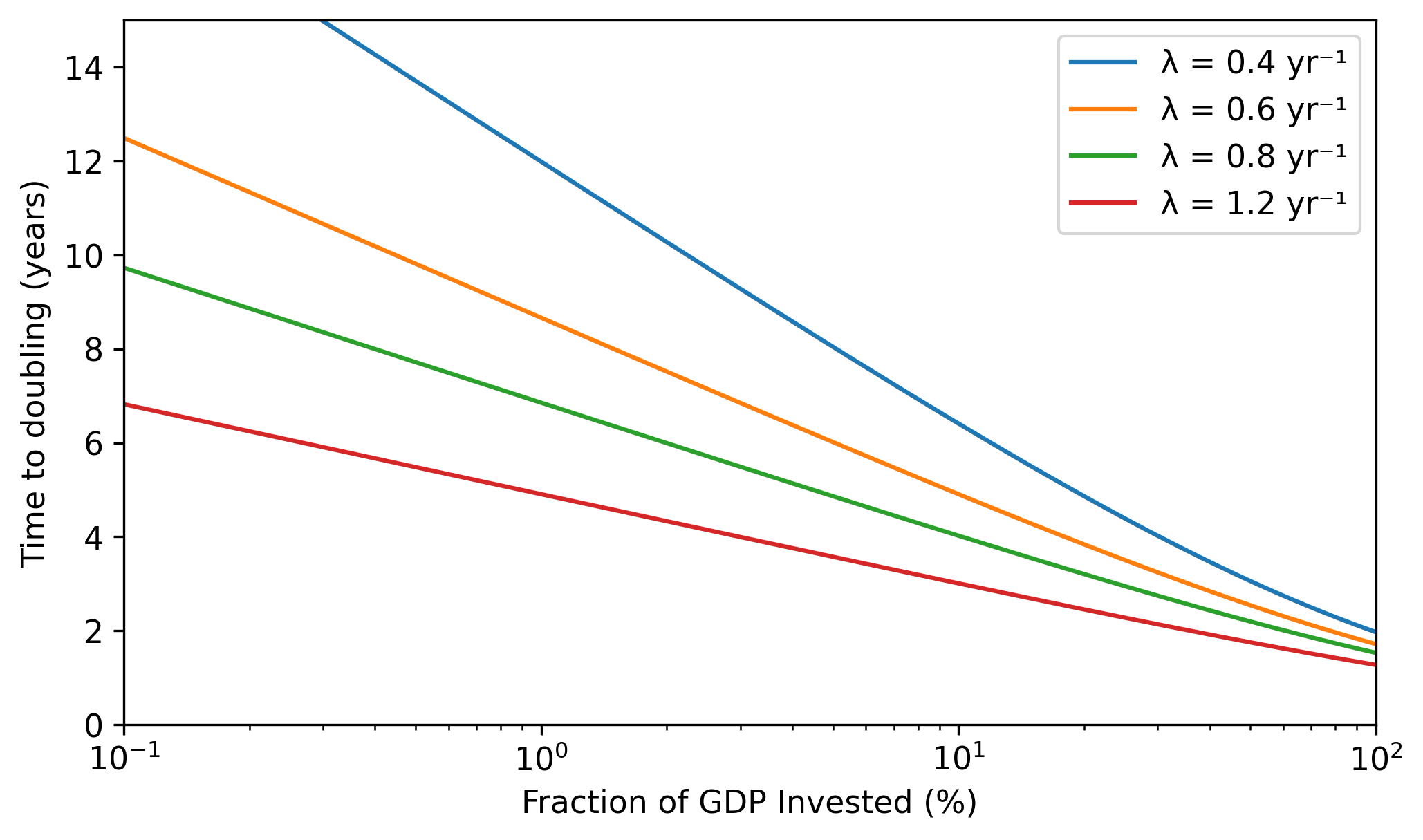
How large could \(f\) be? US gross private domestic investment is about 18% of GDP. Of this, about 13% goes toward physical capital such as structures, equipment, and housing. The remainder of economic activity produces consumer goods and services that would not be useful for the autonomous sector, so 13% represents a rough upper bound on \(f\). At \(f = 0.13\) and \(\lambda = 0.6\) yr\(^{-1}\), the economy would double in about five years.
Lower investment rates increase the time to double, but because \(t^*\) is logarithmic in \(f\), the effect is weak. Even at \(f = 0.001\), just 0.1% of GDP, the economy still doubles in about twelve years.
The economy recomposes itself within a few years
Let's now turn to a more realistic model, using the input-output framework from Part 1 to model the transition to autonomous growth sector by sector. Unlike in the previous section, the model does not artificially distinguish between a rapidly growing sector and the rest of the economy. Instead, each sector produces output using inputs from other sectors, and each sector's output is limited by its installed capital. Different sectors grow at different rates depending on how much existing capacity they have and how much the growing economy demands from them.
Part 1 showed that the economy grows fastest in a particular maximum-growth composition that is heavily weighted toward machinery, metals, and construction. The US economy does not currently have this composition. How fast can it get there?
To answer this, imagine a planning agent that must choose at every point in time which sectors to invest in. There are many objectives the planner could optimize for—maximizing electricity output, or number of shoes, or whatever—but the choice turns out not to matter much. By the turnpike theorem, if the planner is optimizing for growth over a sufficiently long horizon, then regardless of which sector they ultimately want to grow, the best strategy is to funnel investment into the fastest overall growth mode first and redirect production only at the end. The economy converges to the maximum-growth composition from Part 1, and does so quickly. The full formulation is in Appendix D.
Of course, if we naively let the planner maximize growth with no other constraints, it would stop producing essential goods and services. I therefore hold current consumption fixed, so that living standards remain constant. Later sections relax this by allowing consumption to grow and introducing savings constraints. I also hold net exports fixed. Existing trade continues, but all new production above the current baseline comes from domestic capacity and is reinvested domestically.
As in Part 1, the results depend on the cost of substituting capital for labor and how intensively existing capital is utilized. Let us consider three scenarios:
- Free labor: labor is costless, capital at current utilization.
- Priced labor: labor replaced by capital at the costs estimated in Part 1, current utilization.
- Priced labor, emergency utilization: same labor costs, but all capital operates 24/7.
I use the 71-sector BEA summary system (the 398-sector detail tables from Part 1 make solving for optimal growth impractically slow). The maximum-growth rates for the three scenarios are:
| Scenario | \(\lambda^*\) (yr⁻¹), 71-sector | \(\lambda^*\) (yr⁻¹), 398-sector (Part 1) |
| Free labor | 0.57 | 0.61 |
| Priced labor | 0.53 | 0.56 |
| Priced labor, emergency util. | 0.71 | 0.79 |
The 71-sector rates are slightly lower than Part 1's because of the coarser aggregation, but the difference is small.
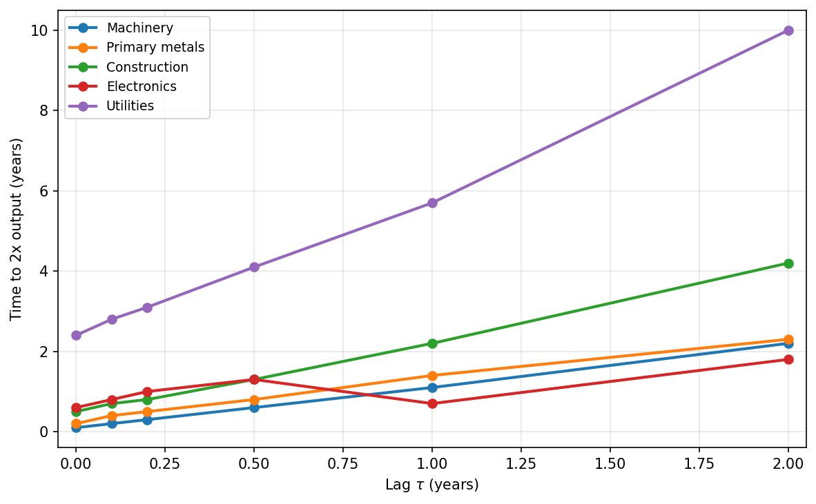
There is no single "economy doubles" milestone, because different sectors grow at very different rates. Figure 2 shows how four key sectors scale over time. Machinery and primary metals double in months, construction is somewhat slower, and utilities are slowest to grow. The first two sectors double quickly because current US production is very low compared to what rapid growth demands. Utilities is slow to scale both because energy production is already a large fraction of the economy, so there is less slack to redirect, and because power generation is very capital-intensive to expand.
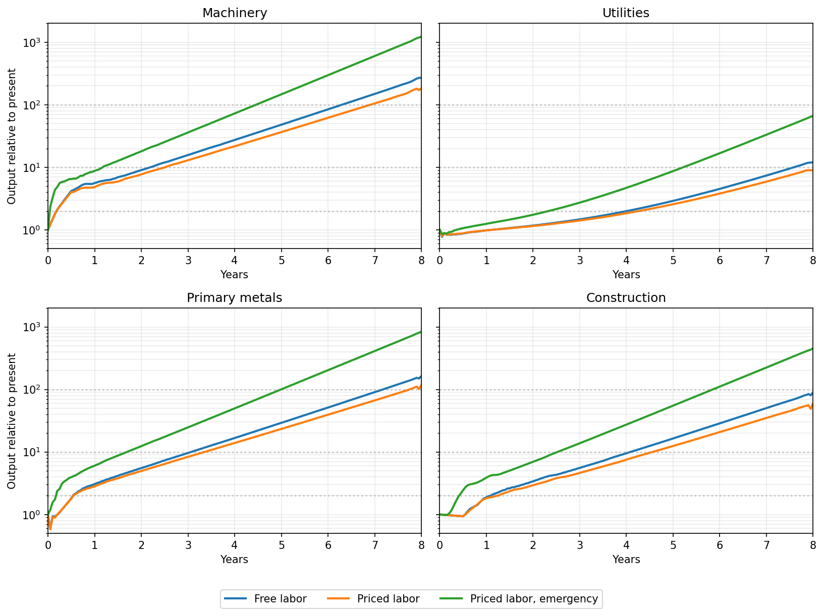
Because energy is required to produce everything, utilities growth is probably the best single proxy for overall economic size. The table below shows when utilities output reaches successive doublings:
| Free labor | Priced labor | Priced, emergency | |
| 2× | 4.1 | 4.3 | 2.4 |
| 4× | 5.8 | 6.2 | 3.8 |
| 8× | 7.2 | 7.7 | 4.9 |
As in Part 1, labor costs have only minor effects on the timeline. Increased utilization, by contrast, greatly decreases the time required to double. In all three scenarios, the first doubling of utilities takes several years but second doubling is much quicker; the time from the second to the third doubling is close to the time to double under maximum growth. After a few doublings, the economy has largely converged to the maximum-growth composition and Part 1's analysis applies directly.
In Figure 3 we plot the robot population over time. It grows from near zero to tens of millions within the first few years, and into the hundreds of millions by year 8 under emergency utilization.
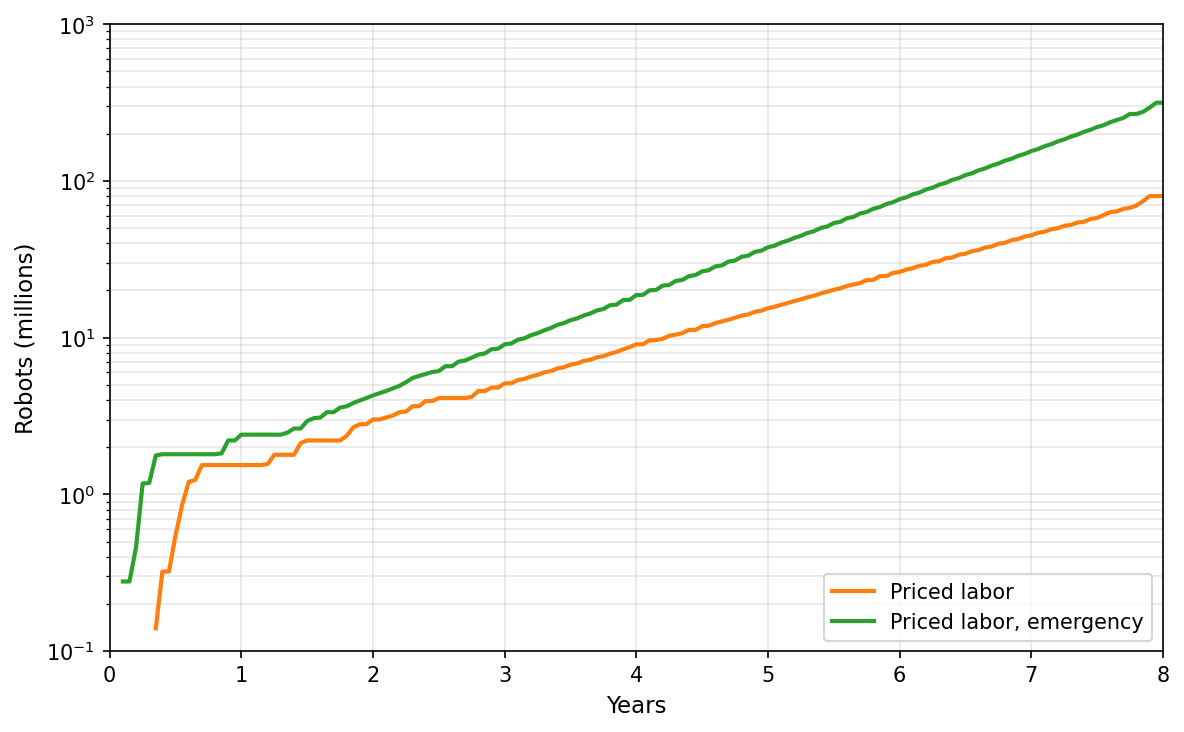
As a sanity check, Epoch AI (2025) approaches the same question from the supply side, with a bottom-up analysis of humanoid component supply chains. They find 2030 production rates of 5–15M humanoids per year plausible under aggressive demand-shock assumptions, with reference-class doubling times of 10–16 months for mature robot categories. Our model passes 20M robots around year 4 and reaches hundreds of millions by year 8 under emergency utilization, with a steady-state robot doubling time of roughly 1 year. The two trajectories are broadly comparable up to the point where the real economy substantially expands, showing that our model's initial robot ramp-up is not manifestly insane (with allowance for an initial delay while the first robot factories come online). The number of robots needed to automate manufacturing is not large; in a rapidly growing economy the robot capital stock is small, and making robots is not a significant constraint relative to producing energy and raw materials.
Construction lags slow the transition but do not change the timescale
The baseline model assumes new capital is productive immediately. In practice, building a factory or power plant takes time: months for equipment installation, years for large structures. I model this as a pure delay: investment at time \(t\) draws resources immediately but the resulting capital appears \(\tau\) later.
To see the effect, I apply a uniform construction lag \(\tau\) across all sectors in the emergency utilization scenario (priced labor, 24/7 operations) and re-solve the transition linear program. Figure 4 shows the resulting sector trajectories for several values of \(\tau\).
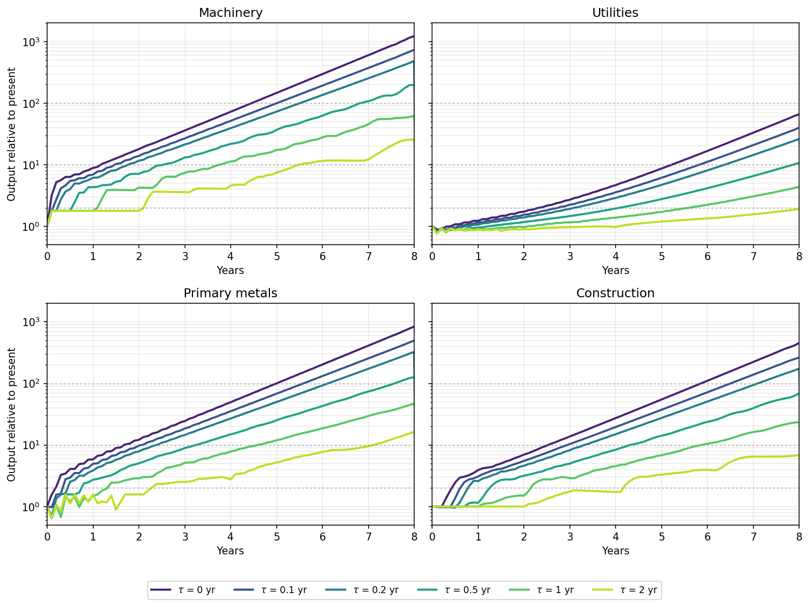
As expected, lags push back all sector trajectories. They both slow the recomposition of the economy toward the maximum-growth composition and reduce the growth rate achieved once it gets there.
Figure 5 shows how long it takes for different sectors to double as a function of the lag. The time to double is roughly linear in the lag, but the slope differs across sectors.
What is a realistic value of \(\tau\)? Current best practice for large industrial facilities is about six months from groundbreaking to operation, though most factories take one to two years. A robot economy with 24/7 construction could plausibly compress these timelines. A lag of 0.5 years for construction and 0.1 years for equipment implies an overall average lag of perhaps 0.3–0.5 years, increasing the time required to double utilities production from 2.4 years to about 4 years.
These estimates are stylized in two ways that push in opposite directions:
- The model assumes a mature automated economy from the start. In practice, there may be an initial period before investors begin redirecting capital toward rapid growth, and early construction lags may be longer than the mature estimate as automated construction techniques are still being learned. Both effects would add time.
- The model assumes a transition from present-day conditions. By the time AGI enables full automation, the economy will likely have already shifted substantially toward automation and capital goods production. This would shorten the transition.
A more realistic model would incorporate both effects, but doing so requires assumptions about the pace of AI deployment and the degree of pre-AGI capital reallocation that are at least as uncertain as the construction lags themselves. We leave this for future work.
Cannibalization of existing capital does not significantly accelerate the transition
The economy starts with roughly $50 trillion in fixed assets. Most of this is in sectors that are overbuilt relative to maximum growth — housing, commercial real estate, retail, healthcare. Could repurposing this stock accelerate the transition?
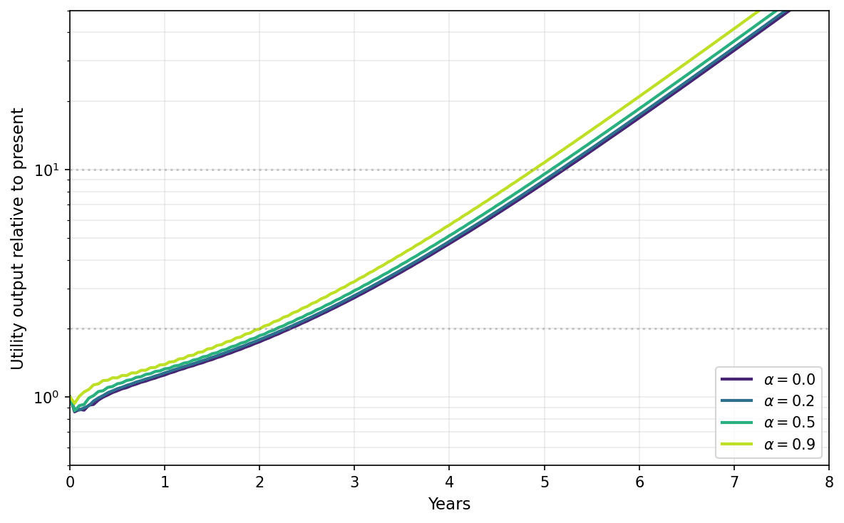
We model this by allowing the optimizer to demolish existing capital and reallocate its components. Each sector's capital is composed of high-level inputs — construction, machinery, electronics, and so on — in proportions recorded by the capital-composition matrix \(\hat{B}\). Demolishing a sector's capital returns these components to the production system as supply available for new capital formation. Recovering the construction component of a car factory, for instance, is equivalent to freeing up that much construction-sector output for use elsewhere — whether by repurposing the building or by scrapping it and rebuilding. In practice, reallocated capital is worth less than freshly produced capital: the building may be poorly suited to its new use, or the machinery may need to be broken down for parts rather than reused directly. We represent this with a recovery fraction \(\alpha\).
In Figure 6, we show how varying \(\alpha\) affects the growth of the utilities sector. The effect is small — at most a few months even when \(\alpha = 0.9\), which is unrealistically high. There are two reasons. Most existing capital is in use producing goods that people need, so the planner cannot free it up without reducing living standards. And most of the overbuilt capital stock is in things like housing, which is not useful for building factories regardless of whether it can be freed up. Durable goods are less than 2% of total consumption, and when we allow them to be deferred we find the effect is negligible.
Consumption growth does not prevent a rapid transition
The baseline model holds consumption fixed at today's level. Nobody starves, but nobody gets richer either. In practice, some of the economy's growing output would go to consumption rather than reinvestment, slowing the transition. How much depends on the savings rate, which, unlike the other parameters in this analysis, is not determined by the production structure itself.
The standard economic approach is to solve a Ramsey problem: choose a savings rate at each point in time to maximize discounted utility. This is difficult to solve jointly with the full IO transition linear program. But the deeper issue is that we have no good reason to trust any particular model of savings. A military buildup or geopolitical race would drive very high savings rates, as competing powers compound past each other in a few years. A world where rapid growth produces valuable new consumer goods would pull savings rates down. So would a world where existential risk makes the future feel uncertain. The Ramsey framework requires specifying a discount rate and elasticity of marginal utility, and it is not clear how to choose these parameters—or, indeed, that the framework itself is the right model for savings behavior in a rapidly transforming economy.
Given this uncertainty, we do not attempt to solve the full Ramsey problem. Instead, we consider two simplified models that bracket a range of reasonable behavior:
- Consumption grows at a fixed rate \(g_c\) per year, regardless of how fast the economy grows.
- The savings rate is fixed at \(s\), so consumption grows as a fixed fraction of GDP.
In both cases we hold the current consumption basket fixed, and assume all consumed goods scale in proportion to one another.
First, suppose consumption grows at a fixed rate \(g_c\). Mandating immediate consumption growth is infeasible — several sectors currently devote their entire net surplus to consumption, leaving no room for simultaneous growth in all of them. I therefore introduce a one-year delay before consumption growth begins, giving the economy time to build capacity.
Figure 7 shows how \(g_c\) affects the time required to double energy production. Even at \(g_c = 0.20\) yr⁻¹, utilities still doubles in about 3.2 years, compared to 2.4 years without any consumption growth. Growth rates above about \(g_c = 0.25\) yr⁻¹ are infeasible without a longer delay.
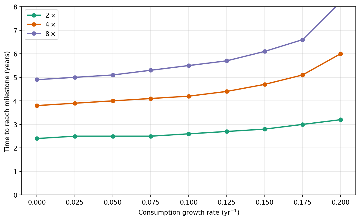
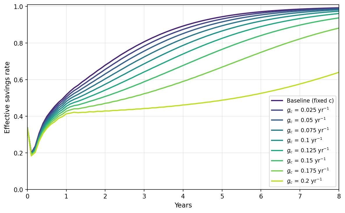
Figure 8 shows the effective savings rate over time under this constant growth rate formulation. At realistic consumption growth rates the savings rates required to drive the transition are high but not crazy: at \(g_c = 0.10\) yr\(^{-1}\) the savings rate sits around 50% for the first two years before climbing, and at \(g_c = 0.20\) yr\(^{-1}\) it stays around 40% for the first few years. Higher consumption growth mechanically leaves less output available for investment, so the effective savings rate is lower. As the economy grows, output increasingly outpaces consumption and the effective savings rate rises. The baseline (no consumption growth) climbs fastest, passing 60% by year 2 and approaching 90% by year 4 — but no real economy would hold consumption pinned for that long, so the realistic envelope is somewhere between \(g_c = 0.05\) and \(g_c = 0.20\).
Now turn to the second case, where the savings rate is held fixed at \(s\). A fraction \(s\) of GDP is invested and the remainder goes to consumption. Applied naively, this can lead to consumption falling below today's level in the first couple of years, while the economy is still small and recomposing. I therefore also enforce that per-sector consumption cannot fall below today's level. In other words, \(s\) is the maximum savings rate, but if maintaining present-day consumption requires saving less, the effective savings rate will be lower.
Figure 9 shows the result. At \(s = 0.50\), the utilities sector doubles in about 2.6 years. At \(s = 0.30\), roughly today's gross savings rate, it doubles in about 3.8 years. Even at \(s = 0.20\), where 80% of GDP goes to consumption, the utilities sector still doubles in under six years. Above \(s \approx 0.7\), the consumption constraint is slack and the economy is bottlenecked on capital formation rather than savings.
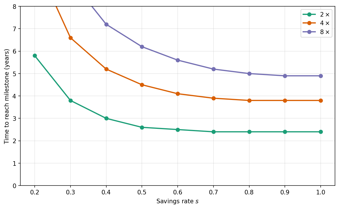
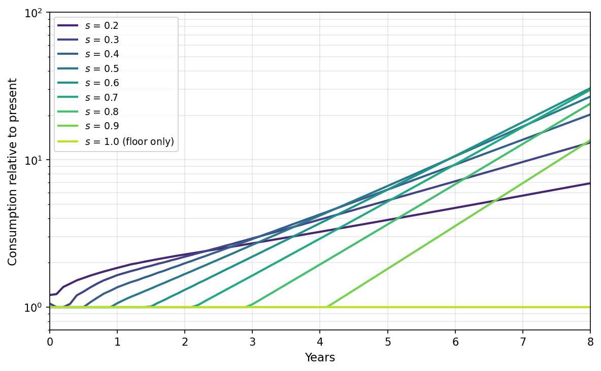
Figure 10 shows how consumption grows over time at each savings rate. Higher savings rates delay consumption growth but produce much more consumption in the long run, because the economy compounds faster. Savings rates of 60–80% overtake the low-savings paths within a few years and reach far higher levels by year 8.
The previous sections examined construction lags and consumption separately. The table below combines them, showing how long it takes for utilities output to double under different combinations of savings rate and construction lag. All results use emergency utilization with central labor cost estimates.
| \(\tau = 0\) | \(\tau = 0.3\) yr | \(\tau = 0.5\) yr | \(\tau = 1.0\) yr | |
| \(s = 1.0\) | 2.4 | 3.5 | 4.1 | 5.6 |
| \(s = 0.70\) | 2.4 | 3.5 | 4.1 | 5.7 |
| \(s = 0.50\) | 2.6 | 3.7 | 4.3 | 5.8 |
| \(s = 0.30\) | 3.8 | 4.7 | 5.3 | 6.7 |
Combining construction lags with realistic savings rates, the utilities sector doubles in roughly 4–5 years across the most plausible parameter combinations. Even at a conservative 30% savings rate and one-year lag, it still doubles within 7 years. It is hard to see timelines stretching much beyond this without postulating very long construction lags or very low savings rates.
Savings rates above about 70% do not result in faster growth — the economy is bottlenecked on how fast capital-goods sectors can physically expand, not on the share of output available for investment.
The second doubling is considerably faster than the first:
| \(\tau = 0\) | \(\tau = 0.3\) yr | \(\tau = 0.5\) yr | \(\tau = 1.0\) yr | |
| \(s = 1.0\) | 3.8 | 5.2 | 6.0 | 7.8 |
| \(s = 0.70\) | 3.9 | 5.3 | 6.0 | 7.9 |
| \(s = 0.50\) | 4.5 | 5.8 | 6.6 | 8.4 |
| \(s = 0.30\) | 6.6 | 7.8 | 8.5 | >10 |
At a 50% savings rate and half-year lag, the first doubling takes 4.3 years, but the second takes only an additional 2.3 years, approaching the maximum-growth rate from Part 1.
Appendix D: The transition formulation
D.1 The transition linear program
The transition problem starts from today's US output vector \(y(0) = y_0\) and asks: what is the fastest feasible trajectory toward maximum growth?
In the language of Appendix A, the planner chooses \(\dot{y}\) at each moment — how fast to grow or shrink each sector. The material balance constrains this choice: investment demand cannot exceed the surplus after intermediate inputs, depreciation, and consumption are covered:
\[
B\dot{y} \leq (I - A - \Delta)\, y - c_0.
\]
In addition, gross investment in each commodity must be non-negative:
\[
B\dot{y} \geq -\Delta\, y.
\]
These two constraints define a linear program that we could solve directly. But this formulation is not rich enough for the transition problem, because it does not track capital explicitly; each sector's capital stock is instead inferred from its output as \(K_j = k_j y_j\). This means there is no way to represent a factory running at higher utilization, where the same capital provides more output. Nor is there an option for a factory to sit idle, even if the factory is consuming valuable inputs while producing useless outputs.
Instead, we track the capital stock \(K\) directly. At each moment, the planner has a fixed amount of capital in each sector and makes two choices: how much of each sector's capacity to use (the output \(y\)), and how much new capital to build in each sector (the investment \(\dot{K}\)). Output can range from zero up to the sector's installed capacity; the planner is free to idle any sector entirely.
We measure \(K\) in output-capacity units: \(K_j\) is the maximum output that sector \(j\)'s installed capital can produce (at the utilization benchmark under consideration). The capacity constraint is then simply
\[
0 \leq y \leq K.
\]
To express the material balance in terms of \(K\), we need the capital-composition matrix \(\hat{B}\), which records what each sector's capital is made of. We construct it from the capital-requirements matrix \(B\) by normalizing each column by the capital-output ratio \(k_j = \sum_i B_{ij}\):
\[
\hat{B}_{ij} = B_{ij} / k_j, \qquad \hat{\Delta}_{ij} = \Delta_{ij} / k_j.
\]
Columns of \(\hat{B}\) sum to one. \(\hat{\Delta}\) is the analogous depreciation-composition matrix.
The material balance becomes: investment demand must not exceed net output after intermediate inputs, depreciation replacement, and consumption:
\[
\hat{B}\,\dot{K} \leq (I - A)\, y - \hat{\Delta}\, K - c_0.
\]
And gross investment must be non-negative:
\[
\hat{B}\,\dot{K} \geq -\hat{\Delta}\, K.
\]
On a maximum-growth path where the capacity constraint is exactly binding (\(y = K\)), this reduces to the output-only formulation and gives the same asymptotic growth rate.
Together these constraints define the set of feasible trajectories. The planner must choose among them by specifying an objective. Many objective functions are possible — maximizing output of a particular sector, or total dollar output — but the precise choice matters little. The turnpike theorem (Dorfman, Samuelson, and Solow (1958); McKenzie (1976)) tells us the optimal path is to recompose the economy toward the fastest-growing composition — the Perron eigenvector \(y^\star\) from Part 1 — ride exponential growth along it, and only redirect toward the specific target at the end.
We use a maximin objective: maximize a scalar \(z\) subject to
\[
y(T) \geq z \cdot y^\star,
\]
which pins the terminal composition to the Perron eigenvector and causes the planner to converge to it rapidly. We solve the resulting continuous-time linear program numerically over a finite horizon using a trapezoidal discretization scheme.
D.2 Construction lags
The baseline model assumes new capital is productive immediately. In practice, building a factory or power plant takes time. We model this as a pure delay: investment at time \(t\) draws resources from the material balance immediately, but the resulting capital appears at time \(t + \tau\), where \(\tau\) is a per-sector lag vector. For \(t < \tau_j\), there is no pre-existing pipeline of investment. The material balance itself is unchanged — resources are consumed when the investment is made, not when the capital comes online.
D.3 Capital reallocation through cannibalization
The baseline model has no mechanism for actively scrapping capital. Cannibalization adds one: a demolition rate \(d \geq 0\) that the planner can choose at each instant, representing how aggressively each sector's existing capital is being torn down.
Demolition removes capital from the source sector and returns a fraction \(\alpha\) of its components to the production system. The modified material balance is:
\[
\hat{B}\,\dot{K} - \hat{B}\,\operatorname{diag}(\alpha)\,d \leq (I - A)\,y - \hat{\Delta}\,K - c_0.
\]
D.4 Consumption formulations
We use two consumption formulations that bracket the range of reasonable assumptions.
The exogenous consumption floor holds consumption at the present-day vector \(c_0\), optionally growing it at rate \(g_c\):
\[
c(t) = c_0\, e^{g_c\, (t - t_d)^+},
\]
where \(t_d\) is a delay before growth begins. This fixes both the level and composition of consumption — the planner must produce at least \(c(t)\) component-wise regardless of whether any good is a bottleneck. The linear program becomes infeasible as \(g_c\) approaches \(g^\star\).
The aggregate fixed savings rate caps total investment at a fraction \(s\) of GDP:
\[
\mathbf{1}^\top (\hat{B}\,\dot{K} + \hat{\Delta}\, K) \leq s\, \mathbf{1}^\top (I - A)\, y,
\]
where the left side is gross investment (net capital formation plus depreciation replacement) and the right side is \(s\) times GDP. The material balance retains the per-sector consumption floor \(c_0\) separately, so that consumption cannot fall below today's level. In effect, \(s\) is a maximum savings rate: if maintaining today's consumption already requires saving less than \(s\), the effective savings rate will be lower. The composition of additional consumption (beyond the \(c_0\) floor) follows today's consumption basket.