
Need for speed
In previous posts I argued that we will soon have a lot of AI workers. Here we look at how fast each of them will be. There is a big difference between a million AI workers plodding along at human speed and “only” ten thousand that each work a hundred times faster.
In short, today’s AIs perform the tasks they can do about ten times faster than humans. At the point they can do human work in general, I expect individual copies would work at closer to human speed, though they would still finish long tasks considerably faster by working around the clock and splitting work across copies. Suitable hardware could raise their raw speed to perhaps a thousand times that of humans.
How fast do AIs run today?
Language models produce text by sequentially generating tokens, each corresponding to about three-quarters of a word. Here is how fast providers read and write tokens for a single user, as measured by Artificial Analysis in October 2026:
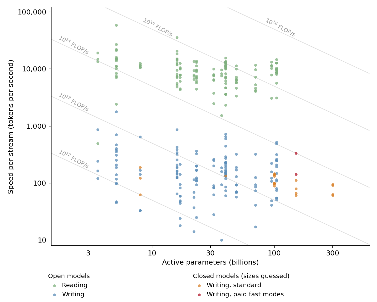
Most models write around 50 to 300 tokens per second whatever their size and read inputs fifty to a hundred times faster, as estimated from the time to the first output token. Reading is much faster than writing because models can process all of their input tokens in parallel, but must generate output tokens one after another. We discuss how tokens are generated in more detail in Appendix A.
Token speed is the most straightforward measure of how fast a language model runs, but it says little about how much work the model gets done. Small models like Haiku or Luna produce tokens much faster than beefy ones like Astra or Fable, but each token is worth less. For this reason, I’m skeptical of naive comparisons of AI and human speed that equate token for “token” (whatever that means for humans). A small model can produce vast quantities of AI slop far more quickly than a human can write, but that is no more interesting than observing that a program spitting words out at random can generate “text” billions of times faster than a human.
A more useful approach is to compare how fast humans and AIs do the same tasks. In my previous post, I found that when AIs can do human work, they need on the order of \(3\times10^{12}\) floating-point operations (FLOP) per second of human time replaced. This number varies a lot with the task and the model, and the estimates behind it are very noisy, but it is consistent across a broad range of tasks, spanning many domains and time horizons.
Dividing a model’s FLOP per second by this number gives its speed relative to a human. Frontier models compute at around \(3\times10^{13}\) FLOP per second while writing (as can be seen from the grey diagonals in the above plot) and so typically perform output-heavy tasks about ten times faster than humans, ignoring gains from parallelizing work across agents. Those same models read tokens at above \(10^{15}\) FLOP per second, and so on reading-heavy tasks can perform hundreds of times faster than humans.
In my post on AI compute, I estimated that if we develop AI systems capable of doing human work in the near future, they will require \(10^{13}\) to \(10^{14}\) FLOP per second of human time; this is somewhat higher than existing tasks, because mean costs are dominated by those tasks that are relatively expensive. As we discuss in Appendix A, such models would probably run at a similar number of FLOP per second as today’s models, since these speeds are set by the hardware they run on. They would therefore perform output-heavy work at roughly human speed, while reading inputs a hundred times faster than humans.
Despite not being much faster than humans at writing, these AIs would still work much faster overall. Reading is a substantial fraction of most jobs, so reading a hundred times faster could roughly double their speed, and working around the clock rather than a 40-hour week gives another factor of about four. Together these would make AI workers about ten times faster than humans.
Probably the most important effect, though, is that AI systems can split work across many copies. You may have already witnessed this if you’ve used Claude Code recently to ask a seemingly straightforward question only to discover, half an hour and several hundred dollars later, that Claude had set up fifty subagents to meticulously investigate each individual proposed Iberian–Basque cognate. In principle, humans could also divide work in this way, but coordination overheads, like the fact you cannot easily hire 100 contractors and then fire them an hour later, make this impractical. On tasks that allow suitable parallelism, AIs could act hundreds of times faster than humans can.
Speed vs utilization
Providers charge more for faster services. OpenAI normally serves GPT-6.1 Sol at around 80 tokens per second, but offers services two and four times faster for twice and six times the price. Anthropic likewise charges twice as much for a fast mode of Claude Opus 5.5 that it says writes up to 2.5 times faster.
These speedups are possible because providers can trade off their hardware utilization, the fraction of the time their GPUs spend doing arithmetic, against speed per user by changing how they batch users and distribute them over GPUs. Batching lets you serve more users at once, which increases utilization but slows down each user. Splitting a model across many GPUs serves each user faster, but the GPUs then spend more time communicating with each other. We discuss how this works in Appendix A.
Typical tradeoffs between utilization and speed per user look something like this:
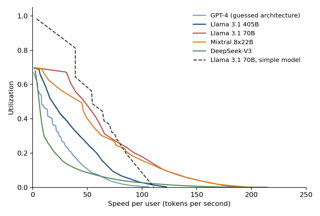
The dashed line shows the simple model we develop in Appendix A for Llama 3.1 70B. The other curves show the model of Erdil (2025) for models served on H100s, which includes more architectural detail and also speculative decoding, a method that lets a model generate several tokens per pass and in practice makes it about two times faster.
Judging by prices and published statistics, providers usually serve models in the middle of these curves, trading off utilization and speed roughly evenly. DeepSeek’s serving statistics imply a utilization of around 10%.
Suppose you have a fixed number of chips. How fast should you run your AIs? The chips’ total output, in tokens per second, is proportional to their utilization \(u(s)\), and each AI running at speed \(s\) takes \(s\) of it, so the number of AIs you can run is
\[N \propto \frac{u(s)}{s}.\]As a simple model, suppose the rate at which they get work done on a project is
\[W \propto s \times N^{\alpha} \propto s^{1-\alpha} \times u(s)^{\alpha},\]where \(0 < \alpha < 1\) captures the diminishing returns to adding more AIs. For Llama 3.1 70B on H100s, using Erdil’s utilization curve, the rate of work at each speed is:
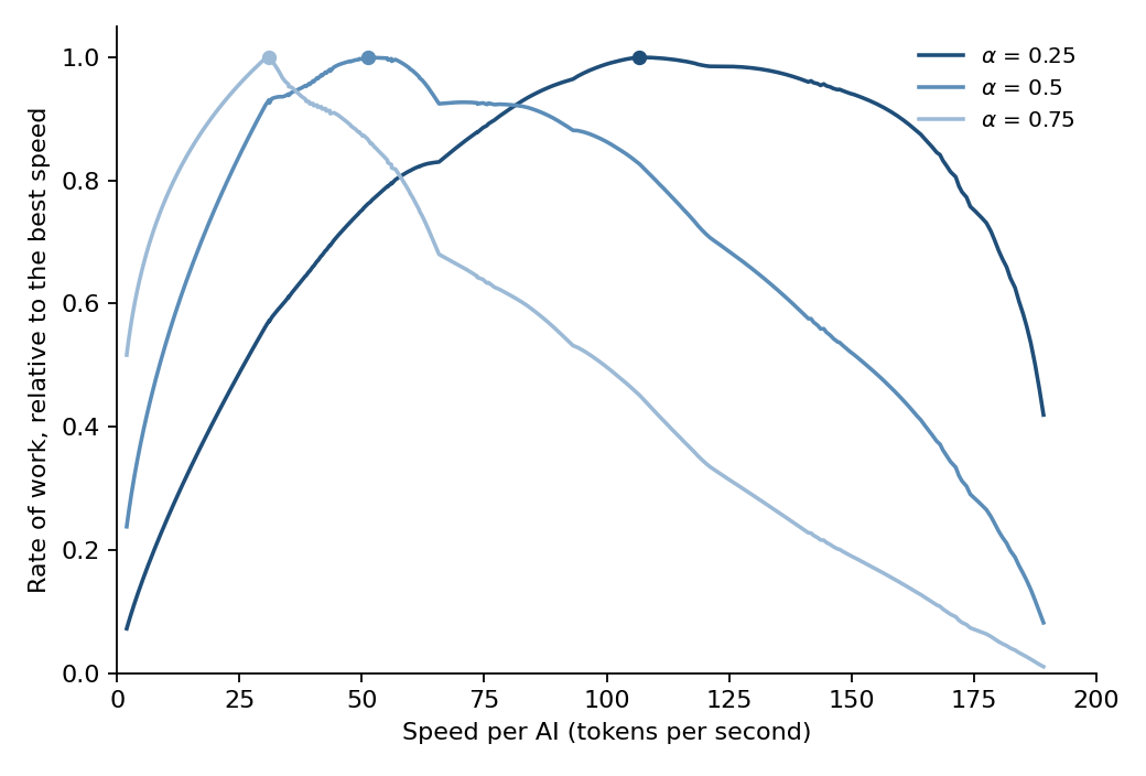
If the work parallelizes well, with \(\alpha\) near one, it is best to run AIs slowly to maximize utilization, but for serial work with \(\alpha\) near zero, it is best to run them as fast as possible.
How fast could future AIs run?
Today’s speeds are set by GPUs, which are designed to serve many users cheaply rather than one user fast. Even at almost zero utilization, they serve large models at no more than a few hundred tokens per second. Hardware built for speed could be much faster.
In Appendix B, we estimate how quickly models could be served on hardware optimized for speed. Even with heavy optimization, a number of steps must happen in sequence in each layer of the model, and the time these take is set by the hardware’s clock speed, which is in turn limited by the physics of silicon transistors.
At today’s clock speeds, on hardware that is otherwise optimistically designed but not wired around a particular model, we estimate these steps take at least about 1 µs per layer, suggesting maximum speeds of
\[\begin{gathered} \text{max token speed} = \frac{1}{L\,t_{\text{layer}}} \approx 10{,}000\ \text{tokens/s} \times \left(\frac{100}{L}\right) \times \left(\frac{1\ \mu\text{s}}{t_{\text{layer}}}\right), \\ \text{max FLOP speed} = \frac{2P}{L\,t_{\text{layer}}} \approx 2 \times 10^{16}\ \text{FLOP/s} \times \left(\frac{P}{10^{12}}\right) \times \left(\frac{100}{L}\right) \times \left(\frac{1\ \mu\text{s}}{t_{\text{layer}}}\right), \end{gathered}\]where \(L\) is the number of layers, \(t_{\text{layer}}\) is the time per layer, and \(P\) is the number of active parameters. Even allowing higher clock speeds or hardware wired around a single model, I think going much faster than this is probably not feasible.
Hardware that could run models approaching these speeds doesn’t exist today, and designing it would take substantial engineering. But, as we discuss at the end of Appendix B, tokens served on it would probably cost several times more than on GPUs, not orders of magnitude more.
If human-level AI requires a model with roughly a trillion active parameters and a hundred layers, and \(10^{13}\) to \(10^{14}\) FLOP per second to match a human, then on such hardware it would perform tasks a few hundred to a few thousand times faster than a human could. Getting beyond this with faster hardware seems very hard.
Alternatively, models might match human performance with substantially fewer FLOP. For this to make them much faster at fixed depth, they would have to produce fewer tokens per second of human work replaced. Working at ten thousand times human speed, for example, would mean matching each second of human work with a single token, assuming the depth remains at a hundred layers. When humans are typing or speaking, they produce about a token per second, so replicating that work with fewer tokens seems quite difficult.
Decreasing model depth could also increase speed, but the room for this is limited. The model we assumed is already only about a hundred layers deep, and some depth is presumably needed to do the relevant calculations. Perhaps a looped architecture, which uses calculations from previous tokens more extensively, could reduce the depth needed somewhat further.
These speeds stack with the advantages from the first section. Reading faster and working around the clock add roughly another factor of ten, and parallelism more on tasks that can be split up. On the right hardware, AIs could do human work thousands to tens of thousands of times faster than people.
Appendix A: How tokens are generated
In this appendix, we develop a simple model of how fast a language model generates tokens on GPUs. We ignore the additional complications that come from the KV cache, mixture-of-experts routing, and other architectural details. The interested reader can find a more detailed treatment in Erdil (2025) or Reiner Pope’s conversation with Dwarkesh Patel.
Outputs from a single GPU
Start with the simplest case, a model with \(P\) parameters running on a single GPU. Suppose that each parameter is stored in one byte, so that the weights take up \(P\) bytes, and that they fit in the GPU’s memory. Each pass requires the GPU to do two things. First, it must read every weight out of its memory and onto the chip where the arithmetic happens, which takes a time
\[t_{\text{read}} = \frac{P}{B},\]where \(B\) is the rate at which the GPU reads from memory, in bytes per second. Second, it must use every weight in one multiplication and one addition for each user it is serving, which takes a time
\[t_{\text{arith}} = \frac{2bP}{C},\]where \(C\) is the rate at which the GPU does arithmetic, in operations per second, and \(b\) is the batch size, the number of users served at once. For a single user, \(b = 1\).
Naively, the time per step would be \(t_{\text{read}} + t_{\text{arith}}\). However, the GPU can read and calculate in parallel, such that the total time per step, \(t_1(b)\), is roughly determined by whichever of these processes is slower:
\[t_1(b) \approx \max\left(t_{\text{read}},\, t_{\text{arith}}\right) = P \max\left(\frac{1}{B},\, \frac{2b}{C}\right).\]The GPU is memory-limited if the batch is smaller than
\[b_* = \frac{C}{2B} \approx 300 \times \left(\frac{C}{2\times10^{15}\ \text{s}^{-1}}\right) \times \left(\frac{3.35\ \text{TB/s}}{B}\right),\]where the reference values are those of an H100. Below \(b_*\), every step takes time
\[t_1(b) \approx \frac{P}{B} \approx 21\ \text{ms} \times \left(\frac{P}{7\times10^{10}}\right) \times \left(\frac{3.35\ \text{TB/s}}{B}\right) \qquad \text{with }b<b_*\]where the reference model is Llama 3.1 70B. A single user of Llama 3.1 70B on an H100 therefore receives about 48 tokens per second, while the GPU’s arithmetic units sit idle more than 99% of the time.
Each token needs \(2P\) FLOP, so the compute performed for each user is
\[\text{flops/s per user} =\frac{2P}{t_1(b)} \approx 2B \approx 7\times10^{12}\ \text{FLOP/s} \times \left(\frac{B}{3.35\ \text{TB/s}}\right) \qquad \text{with }b<b_*,\]whatever the size of the model. A larger model produces fewer tokens per second, but does proportionately more arithmetic for each one.
The batch size trades speed against efficiency. A natural measure of efficiency is the utilization, the fraction of each step the GPU spends on arithmetic,
\[u = \frac{t_{\text{arith}}}{t_1(b)} \approx \min\left(1,\, \frac{b}{b_*}\right).\]Below \(b_*\), each additional user raises the utilization without slowing anyone down. Above \(b_*\), the GPU is fully used and its output is fixed by the arithmetic, so each additional user just slows everyone down. The best operating point is thus around \(b = b_*\).
One additional effect is that every layer comes with fixed delays that do not depend on how much data is processed. Each step of the layer has to be started, intermediate results pass through the GPU’s memory, and the GPU’s processors have to synchronize before the next step can begin. Together these introduce an additional serial delay, \(t_{\text{fixed}}\), for every layer:
\[t_1(b) \approx \max\left(t_{\text{read}},\, t_{\text{arith}}\right) + L\,t_{\text{fixed}}.\]In typical deployments \(t_{\text{fixed}} \approx 60\) µs, which reproduces the measured speeds of Llama 3 70B on two to eight H100s. For Llama 3.1 70B, this adds 4.8 ms to our previous estimate of 21 ms per token.
Inputs from a single GPU
Before writing anything, the model has to read its input. Each input token has its own vector at every layer, so it needs one multiplication and one addition per weight, just like an output token. Unlike output tokens, though, input tokens are all known in advance, so the GPU can pass all \(N\) of them through each layer together, using each weight it reads for every one of them. Reading the input therefore works exactly like serving a batch of \(N\) users, and takes at least time
\[t_{\text{in}}(N) \approx P \max\left(\frac{1}{B},\, \frac{2N}{C}\right) + L\,t_{\text{fixed}}.\]For inputs longer than \(b_*\) tokens the process is compute-bound:
\[\frac{N}{t_{\text{in}}(N)} \approx \frac{C}{2P} \approx 14{,}000\ \text{tokens/s} \times \left(\frac{C}{2\times10^{15}\ \text{s}^{-1}}\right) \times \left(\frac{7\times10^{10}}{P}\right),\]thus a single user’s input is read \(b_* \approx 300\) times faster than its output is written. In practice the ratio is lower, mainly because measured reading speeds include fixed delays before the first token, and speculative decoding speeds up writing but not reading.
Outputs from multiple GPUs
Now suppose we have multiple GPUs and want to split the calculations among them. This introduces a third time-consuming process, that of transferring data between GPUs. Each transfer takes a time
\[t_{\text{transfer}} = \tau_0 + \frac{2bd}{B_{\text{link}}},\]where \(\tau_0\) is a fixed delay, \(d\) is the length of each user’s vector (assuming two bytes per number), and \(B_{\text{link}}\) is the bandwidth of the link between GPUs, in bytes per second. With typical values,
\[t_{\text{transfer}} \approx 5\ \mu\text{s} + 11\ \mu\text{s} \times \left(\frac{b}{300}\right) \times \left(\frac{d}{8{,}192}\right) \times \left(\frac{450\ \text{GB/s}}{B_{\text{link}}}\right),\]where the reference values are a typical fixed delay, the vector length of Llama 3.1 70B, and the link between H100s in the same server.
The naive way to split the calculations among \(k\) GPUs is to give each one \(L/k\) of the model’s \(L\) layers. Each layer needs the output of the one before, so the GPUs work in turn, with \(k-1\) transfers per token:
\[t_{\text{series}}(k, b) = t_1(b) + (k-1)\,t_{\text{transfer}}.\]This does not speed anything up. In fact, the additional transfers slightly slow each token down. Nor does it increase utilization. Splitting a model this way only makes sense when its parameters do not fit on a single GPU.
Instead, the GPUs can make each token much faster by sharing the work within each layer, with each GPU holding a slice of every layer’s weights. Each GPU then computes a partial result for the whole batch, and the GPUs have to add these up about twice per layer (Shoeybi et al. (2019)), so each token needs \(2L\) exchanges.
An exchange takes two rounds. The batch’s vectors are split into \(k\) pieces, one owned by each GPU. In the first round, each GPU sends every piece to its owner, which adds them up. In the second, each owner sends its finished piece to all the other GPUs. All the GPUs send at the same time, and in each round each one sends and receives \((k-1)/k\) of the batch’s \(2bd\) bytes, so
\[t_{\text{exchange}}(k, b) = 2\tau_0(k) + \frac{k-1}{k} \times \frac{4bd}{B_{\text{link}}(k)},\]where \(\tau_0(k)\) and \(B_{\text{link}}(k)\) are the fixed delay and the bandwidth with which each GPU can send to the other \(k-1\).
GPUs are typically wired together in groups of \(n\), 8 in an H100 server and 72 in a GB200 NVL72 rack. Within a group, the GPUs share a fast switch, so for \(k \le n\) the fixed delay and bandwidth are those of the transfers above, about 5 µs and 450 GB/s on H100s, whatever \(k\) is. An exchange then takes about two transfers however many GPUs share the work. Once \(k\) is larger than \(n\), some of the GPUs are connected by network links, which on an H100 server carry 50 GB/s per GPU, about an order of magnitude less, and have longer fixed delays. Exchanges therefore slow down sharply as soon as they cross between groups, and only gradually after that as more groups are added (Erdil (2025)).
The time per token is
\[t_{\text{parallel}}(k, b) = \frac{\max\left(t_{\text{read}},\, t_{\text{arith}}\right)}{k} + L\,t_{\text{fixed}} + 2L\,t_{\text{exchange}}(k, b).\]Each user then receives tokens at a speed \(s = 1/t_{\text{parallel}}(k, b)\), while each GPU spends a time \(t_{\text{arith}}/k\) of each step on arithmetic, so its utilization is
\[u(k, b) = \frac{t_{\text{arith}}}{k\,t_{\text{parallel}}(k, b)}.\]A provider chooses \(k\) and \(b\). Increasing the number of GPUs makes each user faster, but decreases utilization, as the GPUs must wait for exchanges at each step. Increasing the number of users increases utilization, but slows everyone down, through both the arithmetic and the larger exchanges. Optimizing over \(k\) and \(b\) gives a frontier between utilization and speed per user, which we show below for Llama 3.1 70B with our toy parameters on a single H100 server:
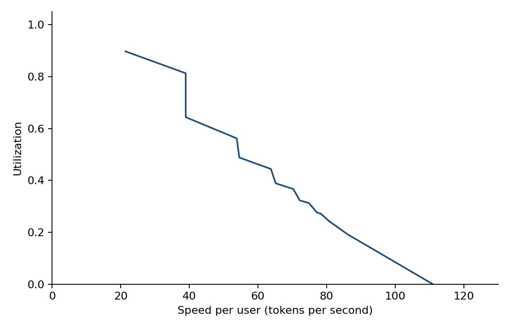
A utilization of about 80% is achieved by using a single GPU to serve \(b_*\) users, each at a speed
\[s = \frac{1}{P/B + L\,t_{\text{fixed}}} \approx 39\ \text{tokens/s}\]for Llama 3.1 70B on an H100. Maximum speed is achieved by serving a single user on all \(n\) GPUs, so that each of the \(2L\) exchanges carries almost no data and takes only its fixed delay \(2\tau_0\):
\[s_{\max} = \frac{1}{P/nB + L \times \left(t_{\text{fixed}} + 4\tau_0\right)} \approx 110\ \text{tokens/s},\]at almost zero utilization.
In terms of compute, each user therefore receives
\[\begin{gathered} \text{flops/s per user} = 2Ps \approx 5\times10^{12}\ \text{FLOP/s} \qquad \text{at 80\% utilization}, \\ \text{flops/s per user} = 2Ps_{\max} \approx 1.5\times10^{13}\ \text{FLOP/s} \qquad \text{at maximum speed}\,, \end{gathered}\]for Llama 3.1 70B. More generally, each token requires reading all the weights, which takes at least \(P/kB\) on \(k\) GPUs, so a user can receive at most
\[\text{flops/s per user} \le 2kB \approx 5\times10^{13}\ \text{FLOP/s} \times \left(\frac{k}{8}\right) \times \left(\frac{B}{3.35\ \text{TB/s}}\right),\]whatever the size of the model.
Appendix B: How fast can you go?
With enough chips, all the work that can be done in parallel takes no time, and the speed of a model is set by the steps that must happen in sequence. Each token passes through \(L\) layers in turn. Within each layer, \(n\) arithmetic operations must happen in sequence, and partial results computed in different places must be gathered together \(k\) times. Each of these steps takes some number of clock cycles, so the time per token is
\[t_{\text{token}} = L \times t_{\text{clock}} \times \left(n \times c_{\text{arith}} + k \times c_{\text{gather}}\right),\]where \(t_{\text{clock}}\) is the duration of one clock cycle, \(c_{\text{arith}}\) is the number of cycles one arithmetic operation takes, and \(c_{\text{gather}}\) is the number of cycles one gathering takes, whether between parts of one chip or between chips.
Clock speed
Modern GPUs run at about 2 GHz, so \(t_{\text{clock}} \approx 0.5\) ns, and the clock speeds of microprocessors have barely risen since the mid-2000s:
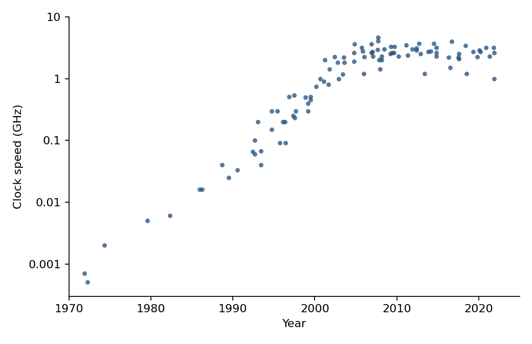
Clock speeds stalled in the mid-2000s because chips reached the limit of how much heat they could shed. A chip’s power grows roughly as the cube of its clock speed, because a faster clock not only means more switches per second but also requires a higher voltage for each switch. Even with unlimited cooling, voltages cannot be raised much beyond present-day values, because the thin insulating layers in transistors would wear out quickly. Someone willing to pay much higher power costs could therefore probably only reach clock speeds of order 10 GHz without switching to fundamentally different physics.
Arithmetic
Each matrix multiplication ends with sums of thousands of numbers, and adding \(d\) numbers in pairs takes \(\log_2 d\) steps however many chips are available. A layer of Llama 3.1 70B has vectors of \(d = 8{,}192\) numbers and contains nine such sums in sequence, which together with about ten other operations make \(n \approx 120\). The exact number varies with architectural choices, and some of these steps can be done in parallel, but I think \(n\sim100\) for any realistic architecture.
On a GPU, an arithmetic operation takes about four clock cycles, so \(c_{\text{arith}} \approx 4\), and the total arithmetic takes about 500 cycles, or 0.2 µs, per layer. But there are faster ways to do the required arithmetic. For instance, summing each digit position of a long series of numbers separately cuts the clock cycles needed for each sum about tenfold. With such tricks, the average operation takes about one clock cycle, so \(c_{\text{arith}} \approx 1\) and the arithmetic in a layer takes roughly 100 clock cycles, or about 50 ns.
Gathering
A layer’s weights are spread across a large area of silicon, and each multiplication happens next to the weight it uses. Each number a layer produces is a sum of thousands of these products, so before the next step can start, the products must be brought to one place and added, and the result sent back out to wherever the next weights are. Some of these sums can happen at the same time, so the number of gatherings that must happen in sequence depends on the architecture and on how the work is laid out. For Llama 3.1 70B on typical hardware, \(k\) is roughly six.
On GPUs, a gathering takes a couple of microseconds, several thousand clock cycles, with software optimized for speed, whether within one GPU (Hazy Research) or between GPUs in a server (Shen et al. (2026)). With standard software, a gathering between GPUs takes closer to 10 µs, so the two in each layer add about 20 µs to the 60 µs fixed delay within each GPU that we used in Appendix A. Gatherings are this slow because GPU processors pass numbers to one another through memory shared across the whole chip, and each trip to that memory takes hundreds of clock cycles.
A faster approach is to send each message directly to where it is needed. However, messages move in short hops between neighboring parts of the chip, with each hop taking at least one clock cycle, and routing a message takes additional cycles. Even chips designed to be very fast, such as Groq’s AI chips and D. E. Shaw Research’s Anton 3, need roughly 50 to 150 clock cycles, around 50 ns, to gather results across one chip (Abts et al. (2020); Shim et al. (2022)), so \(c_{\text{gather}} \approx 100\) within one chip.
For frontier models, a layer is usually too big to fit on one chip. Gatherings therefore require communication between chips, which is slow because signals leaving a chip’s package must pass through a limited number of connections and travel over long, noisy paths, so each connection runs at very high speed through circuits that take tens of nanoseconds to send and decode a message. Crossing between chips takes 55 ns on Anton 3 and 300 ns on Groq’s chips (Bitar et al. (2026)), so a gathering that must cross between chips and back takes several hundred cycles or more. For frontier models we therefore assume about 300 cycles per gathering, roughly Anton 3’s crossing between chips and back plus a gathering within each chip.
The only fundamental limit on gathering is the time it takes a signal to cross the hardware holding a layer. Light crosses a meter in about 3 ns, but signals on a chip typically travel ten or more times slower, so a layer spread over several centimeters of silicon requires at least a few nanoseconds for each gathering.
In principle, hardware could get close to this by wiring each gathering to follow the model’s structure, so that results travel on dedicated wires rather than in hops, and by keeping each layer on a single wafer or package, so that no gathering crosses a slow link between chips. Such hardware could cut a gathering to tens of cycles, but would only perform well for limited model architectures.
Overall speed
Putting the terms together, we estimate that a layer on hardware optimized for latency would take
\[t_{\text{layer}} \approx \left(\frac{t_{\text{clock}}}{0.5\ \text{ns}}\right) \times \left[0.05\ \mu\text{s} \times \left(\frac{n}{100}\right) \times \left(\frac{c_{\text{arith}}}{1}\right) + 0.9\ \mu\text{s} \times \left(\frac{k}{6}\right) \times \left(\frac{c_{\text{gather}}}{300}\right)\right],\]which gives an approximate, optimistic answer of about 1 µs. This is dominated by gathering rather than by arithmetic.
For comparison, the fastest hardware so far is a chip from Taalas, which takes about 2 µs per layer, but for a model small enough to fit on a single chip, Llama 3.1 8B, with its weights printed directly into the chip’s wiring. Cerebras, which builds each chip from a whole silicon wafer, took 17 µs per layer for the same model at its launch, and the fastest GPU runs take about 50 µs.
At what cost?
How much more would it cost to run a model near this maximum speed? Hardware built for it would differ from a GPU in two main ways.
First, its memory. One way to supply the weights fast enough would be to store them in SRAM, the fast memory built into a chip, which costs about ten times as much per byte as the HBM that GPUs use, roughly $100 per GB for TSMC’s densest SRAM at $30,000 per wafer against about $12 for HBM.
This need not raise the cost per token though, because the memory is shared by everyone a copy of the model serves. A fast copy could pipeline users through its layers, so that a hundred-layer model serves a hundred users at 10,000 tokens per second each, about a million tokens per second. A GPU copy of any sufficiently large model produces at most about 10,000 tokens per second, so the hundredfold higher output more than offsets the tenfold higher memory price.
Second, its arithmetic. Each token needs the same arithmetic however fast it is produced. In a simple design that processes one token at a time in each layer, arithmetic sized to finish in a few tens of nanoseconds would sit idle about 95% of the time, waiting for gathering. The hardware could instead carry much less arithmetic, taking about as long as the gathering, which would keep it busy about half the time at the cost of roughly halving the speed.
Keeping the arithmetic busy also requires every layer to be working at once, since each layer’s arithmetic sits on its own chips. This requires pipelining, with a different user in each layer at any moment. Because each user’s data also spends time in transit between layers, filling the pipeline takes somewhat more users than there are layers, and it loses efficiency whenever there are too few users or their traffic is uneven.
The memory and arithmetic of hardware built for speed therefore need not cost much more per token than a GPU’s, provided it can be pipelined efficiently. Its networks and packaging would have to meet much tighter latency requirements, which could make them more expensive, though I don’t know how much. My guess is that tokens served this way would cost several times more than on GPUs, but not orders of magnitude more.
Nobody yet knows how to build such chips, so at present they cannot be bought at any price, and substantial R&D would be needed to create them. The more closely they are tailored to a particular model architecture, the faster they can be and the fewer models they can run. Our estimate assumes chips heavily tailored to the kind of models in use today, but not to a single architecture. In the extreme, the weights can be printed into the chip, as Taalas does, so that each chip runs a single model. The more specialized the chip, the fewer chips its R&D is spread over, and the more value it loses when the models it was built for become obsolete.