In Part 1, I found that a fully automated economy using today's production methods could double roughly every year. In Part 2, I modeled the transition from today's economy to that maximum-growth composition and found that energy production could double within about four years. Both parts held production methods fixed: each sector continues using exactly the recipes it uses today, with robots replacing human workers.
That assumption is too conservative. Today's production recipes were chosen at very different factor prices from what a post-AGI economy would face. Labor is expensive today, so recipes minimize labor use. Humans must also be physically present, so recipes are built around them. Interest rates are low, so recipes lean on durable equipment that lasts for decades. Post-AGI, labor becomes nearly free and capital reproduces fast enough that effective interest rates rise sharply.
This part asks how much faster the economy could grow when recipes are reoptimized for post-AGI factor prices, using only existing or historically-observed technology rather than novel improvements. The first section starts from the US 2017 input-output tables and applies four channels: stripping out the capital and services that exist only to accommodate human workers, closing the productivity gap between average and frontier plants, building cheaper short-lived capital, and shifting recipes toward more labor-intensive production. I also revisit Part 1's construction-lag treatment, as lags become increasingly important at higher growth rates. The second section turns to historical US input-output tables going back to 1947, and asks how much further the rate rises when each commodity can be produced using the cheapest recipe from any era.
This part is a grab bag of different effects, each with its own uncertainties, but that largely stack together. My central estimate is that the economy's maximum self-reproduction rate is between 1 yr⁻¹ and 2 yr⁻¹, corresponding to doubling times of four to eight months. This is roughly twice as fast as Part 1's one-year doubling time. Part 1's savings-rate adjustment applies unchanged. I have not recomputed resource-depletion adjustments on the reoptimized recipe mix; Part 1 shows these are unlikely to overturn the qualitative result, but the exact adjustment may differ because reoptimized recipes draw on a different resource bundle.
Existing or historically-observed methods of production cannot push the rate much higher than this. In Part 4 we will ask: how much faster could production go with better technology?
This series grew out of a project initiated by Holden Karnofsky, with substantial earlier work by Constantin Arnscheidt and Adin Richards. I’m grateful for comments on this post and/or earlier iterations of the project from Holden, Constantin, Adin, Paul Christiano, and Tom Davidson. Thanks also to Claude Opus 4.6 and 4.7 for help with all aspects of this project; in particular, the appendices were written with heavy AI assistance and are less polished than the main text.
Improvements absent technological change
Construction lags become more severe at high growth rates
Part 1 modeled construction lags with two uniform values — one for structures, one for equipment — and found that they reduced the growth rate modestly unless structure lags ran to multiple years. Here we give each sector its own construction lag drawn from industry data on actual build durations, and add a separate deployment lag for heavy-process industries, such as semiconductors, that require substantial post-build commissioning time. We also lag flow inputs through the intermediate matrix, capturing transport and production-cycle times for these goods. We model AGI as eliminating regulatory time entirely and compressing physical durations to the fastest currently-demonstrable benchmarks. Details are in Appendix E.
Why do lags matter more at the higher growth rates we compute in this part? Consider a toy single-sector economy where capital \(K\) produces output at rate \(\mu K\), with all output reinvested as new capital. Without any lag, capital grows exponentially at rate \(\mu\). With a construction lag \(\tau\), so that output produced at time \(t\) becomes installed capital at time \(t + \tau\), capital increases at a rate:
\[
\dot K(t) = \mu K(t - \tau).
\]
Substituting an exponential solution \(K(t) = K_0 e^{\lambda t}\) gives the self-consistent growth rate
\[
\lambda = \mu e^{-\lambda \tau}.
\]
This has two regimes. When the lag is short compared to the doubling time, the growth rate approaches \(\mu\) — the no-lag rate. When the lag is comparable to or longer than the doubling time, the growth rate becomes
\[
\lambda \approx \frac{\log(\mu \tau)}{\tau},
\]
dominated by the lag \(\tau\). The capital efficiency \(\mu\) enters logarithmically and increasing it only marginally increases \(\lambda\). Part 1's growth rates sit in the first regime: lags are short relative to the doubling time, so they cost relatively little. The higher growth rates in this part push closer to the second regime, where lags take a larger bite.
Applying per-sector lags to the full IO model at emergency utilization with priced labor:
| Lag scenario | Growth rate (yr⁻¹) | Doubling time (yr) |
| No lags | 0.82 | 0.85 |
| AGI-compressed lags | 0.68 | 1.02 |
| Current US lags | 0.50 | 1.38 |
Part 1's two-bucket lag model gives 0.63 yr⁻¹ at a 6-month structure lag and 1.2-month equipment lag, close to the 0.68 yr⁻¹ here. Resolving lags per-sector does not substantially change the headline.
Production without humans needs less capital and fewer service inputs
Part 1's Von Neumann calculation already excludes consumer goods, because they do not enter as intermediates in manufacturing; the maximum-growth economy does not invest in them. But human workers also drive costs inside production sectors. For example, if a mining company buys lunch for its workers, this shows up as an intermediate input to mineral ore production. The same firm may need to build office space for its management, use vehicles with driver cabs, and develop HR systems for payroll. All of these capital goods and service expenditures exist only because humans are employed by the company, and once labor is automated, none of it is needed.
In Appendix F.2 we work through every row of the IO system on both channels — \(A\) for intermediate inputs and \(B\) for capital — and compute the contribution of each cut to \(\lambda^*\). The combined effect at the three lag scenarios is:
| Growth rate \(\lambda^\ast\) (yr⁻¹) | No-lag | AGI-lag | US-lag |
| Baseline | 0.82 | 0.68 | 0.50 |
| Capital removed | 0.99 | 0.79 | 0.56 |
| Intermediate inputs removed | 0.98 | 0.78 | 0.56 |
| Combined | 1.15 | 0.88 | 0.61 |
The biggest capital savings come from office and commercial structures that currently house white-collar and retail workers, and are no longer needed once these workers are automated. The biggest intermediate savings are also from office space — when firms lease rather than own, rent appears as a flow through \(A\) rather than as owned capital through \(B\). Beyond offices, the next-largest intermediate cuts are management and administrative services that exist to coordinate human workers.
Closing within-industry productivity gaps modestly speeds up growth
The Von Neumann calculation in Part 1 takes each sector's production recipe to be what the average plant does. But the average plant is not the best plant. Within a typical manufacturing industry, the BLS Dispersion Statistics on Productivity finds that the 90th-percentile plant produces roughly 50% more output per unit of input as the average. AGI plausibly closes most of the real gap by managing every plant at frontier quality and rebuilding capital at the best available vintage.
Not all of the 90-10 spread reflects closeable productivity differences. Bloom et al. (2019) decompose within-industry variation in total factor productivity into contributions from four factors: management practices, R&D intensity, ICT spending, and worker education. AGI plausibly substitutes for each of these. These factors account for about a third of the raw 90-10 spread, with the rest reflecting pricing strategy, location, and measurement noise rather than closeable differences. We apply this third to each manufacturing sector, and a uniform 10% uplift across non-manufacturing. Details are in Appendix F.3.
The harder question is what the productivity gap actually means. A more productive plant might use labor more efficiently, capital more efficiently, or get more output from the same materials. The literature has not directly decomposed cross-sectional plant productivity dispersion into factor-augmenting components. The closest evidence — Doraszelski and Jaumandreu (2018) on the bias of technological change over time — suggests roughly equal labor-augmenting and Hicks-neutral contributions. We adopt a 50/50 split as our central case, noting the uncertainty by reporting bounding cases in both directions.
Computing growth rates under each decomposition, we find:
| Growth rate \(\lambda^\ast\) (yr⁻¹) | No-lag | AGI-lag | US-lag |
| Baseline (no uplift) | 0.82 | 0.68 | 0.50 |
| Labor-augmenting only | 0.82 | 0.68 | 0.50 |
| Central | 0.91 | 0.74 | 0.53 |
| Hicks-neutral only | 0.99 | 0.79 | 0.56 |
The growth effects of labor-augmenting productivity gains are small. Post-AGI, labor is already cheap, so saving more of it adds little. The Hicks-neutral half of the productivity gap drives most of the modest central-case uplift.
Cheaper, shorter-lived capital can substantially increase growth
Capital wears out as you use it. At today's real interest rate of about 5%, durable capital makes sense because the cost of tying up funds is small relative to the savings from not replacing equipment frequently. At doubling times of around a year, the opportunity cost of capital is much higher. A 30-year machine will see the economy grow more than a billion-fold over its lifetime. Almost all of its useful life falls in a period when it is a negligible fraction of the capital stock. The optimal response is to build cheaper, shorter-lived capital.
Reducing capital requirements per unit of output also increases depreciation, because cheaper or less durable equipment wears out faster. At modest reductions (10–20%), the depreciation penalty is small. At larger reductions it grows, and eventually each capital good hits a physical ceiling. We model this tradeoff using a power-law wear function calibrated to BEA depreciation rates, and estimate per-good engineering ceilings for each capital category. The formalism and ceiling values are in Appendix F.4.
At emergency utilization with priced labor:
| Growth rate \(\lambda^*\) (yr⁻¹) | No-lag | AGI-lag | US-lag |
| Baseline | 0.82 | 0.68 | 0.50 |
| 10% less capital, uniform | 0.90 | 0.73 | 0.53 |
| 20% less capital, uniform | 0.97 | 0.77 | 0.55 |
| Per-good engineering ceilings | 1.06 | 0.83 | 0.57 |
| Unconstrained optimum | 1.81 | 1.11 | 0.66 |
I think the 10% uniform scenario is probably conservative, but the per-good engineering ceilings are more aggressive and I'm not sure they can be realized. The unconstrained optimum extrapolates far outside calibrated ranges and is probably very unrealistic. This channel is more uncertain than the previous two. How far each capital good can be compressed is a component-level engineering question, and the aggregate is hard to pin down without detailed analysis of individual goods.
Cheap labor shifts recipes toward labor-intensive production
Every sector can trade capital for labor to some extent, producing with larger workforces rather than investing in labor-saving equipment. Today's recipes are optimized for current US wages and are capital-heavy as a result. Post-AGI, robots and compute replace a human worker at roughly 8% of their current wage, and the optimal recipe in every sector shifts back toward labor.
How much it shifts depends on how easily each sector can substitute labor for capital. Economists usually model this using the constant-elasticity-of-substitution (CES) production function:
\[
Y = \left[\alpha L^{(\sigma-1)/\sigma} + (1-\alpha) K^{(\sigma-1)/\sigma}\right]^{\sigma/(\sigma-1)},
\]
where \(\sigma\) is the elasticity of substitution between labor and capital. At \(\sigma = 0\) inputs are perfect complements: recipes are locked at fixed proportions, and cheap labor delivers nothing. At \(\sigma = 1\) the formula reduces to Cobb-Douglas, \(Y = L^\alpha K^{1-\alpha}\), where each input keeps the same cost share regardless of relative prices. Higher \(\sigma\) means more aggressive rebalancing. Plant-level estimates across manufacturing industries cluster around \(\sigma \approx 0.5\) (Oberfield and Raval (2021), Chirinko (2008)), with a credible range of \([0.3, 0.7]\).
Labor service is supplied by robot and compute capital with fixed engineering coefficients, but the rental cost of that capital depends on the growth rate \(\lambda^*\). The growth rate depends in turn on what recipes every sector chose. So \(\sigma\) is the only free parameter we set, and each sector's recipe falls out of cost-minimization at the converged shadow prices. Details are in Appendix F.5. At emergency utilization with priced labor, the growth rate under different values of \(\sigma\) is:
| Growth rate \(\lambda^*\) (yr⁻¹) | No-lag | AGI-lag | US-lag |
| Baseline | 0.82 | 0.68 | 0.50 |
| \(\sigma = 0.3\) | 1.00 | 0.79 | 0.56 |
| \(\sigma = 0.5\) | 1.16 | 0.89 | 0.61 |
| \(\sigma = 0.7\) | 1.37 | 1.01 | 0.67 |
| \(\sigma = 1\) | 1.85 | 1.28 | 0.82 |
These numbers should not be taken too seriously. The literature estimates of \(\sigma\) come from small wage shifts, presumably vary between sectors, and are being extrapolated across a large price collapse. The CES form also misses labor-intermediate substitution. The lag penalty also widens under CES substitution, because shifting toward labor pulls more weight onto robot and compute capital, which carry their own lag drag. The table is useful as an indication that cheap labor could be a substantial effect, but the magnitude is uncertain.
Summary
Three of the channels above — management, human presence, and durability — modify independent parts of the IO matrix and compose cleanly. CES labor substitution is harder to compose because it rebuilds the system at different factor prices. Of the four, human presence is the one I'm most confident in, as things like office space and corporate services are clearly unneeded in work sites where humans have been automated. Management, durability, and CES labor substitution each depend on parameters with more uncertainty.
The table below stacks each less-certain channel on top of the Part-1-plus-presence baseline, and shows the all-four-combined row at both the central durability setting (\(u = 1.1\)) and the engineering-ceilings upper bound. Growth rates \(\lambda^*\) (yr⁻¹) and doubling times \(T_2\) (months), at emergency utilization with priced labor:
| \(\lambda^*\) (yr⁻¹) | Doubling time (months) | |||||
| Scenario | No-lag | AGI-lag | US-lag | No-lag | AGI-lag | US-lag |
| Baseline | 0.82 | 0.68 | 0.50 | 10.1 | 12.3 | 16.6 |
| + Human presence | 1.15 | 0.88 | 0.61 | 7.3 | 9.4 | 13.7 |
| + Human presence + Management | 1.27 | 0.95 | 0.64 | 6.5 | 8.7 | 12.9 |
| + Human presence + Durability (\(u = 1.1\)) | 1.26 | 0.94 | 0.64 | 6.6 | 8.8 | 13.0 |
| + Human presence + Durability (engineering ceilings) | 1.50 | 1.07 | 0.69 | 5.6 | 7.8 | 12.0 |
| + Human presence + CES labor sub (\(\sigma = 0.5\)) | 1.60 | 1.12 | 0.72 | 5.2 | 7.5 | 11.6 |
| All four combined (\(u = 1.1\)) | 1.94 | 1.28 | 0.79 | 4.3 | 6.5 | 10.6 |
| All four combined (engineering ceilings) | 2.27 | 1.41 | 0.83 | 3.7 | 5.9 | 10.0 |
At AGI-lag, baseline plus human presence reaches 0.88 yr⁻¹ on its own. The all-four-combined row pushes this to 1.28 yr⁻¹ at the central durability setting and 1.41 yr⁻¹ at engineering ceilings.
Older recipes support faster growth
Previous iterations of the US economy had faster growth rates
The US has published input-output tables going back to 1947. Figure 1 shows the free-labor Von Neumann growth rate at several points in time. Over the past seven decades the rate has more than halved, both on the raw matrices and after applying the F.2 human-presence cut to each year's IO matrix.
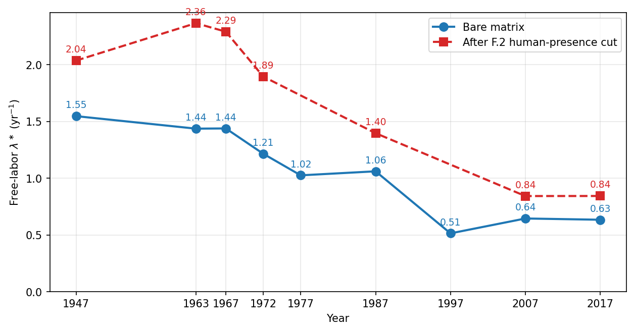
The dominant form of technological progress in manufacturing has been labor-saving capital deepening: replacing workers with more and better machines. This raises output per worker but increases the capital required per unit of output; the Von Neumann growth rate is determined by the latter. The historical labor-intensive recipes use less capital, and at post-AGI factor prices that makes them the cheaper option. A 1947 steel mill that employs fifty workers and ties up less capital per ton of steel is a better deal than a 2017 mill that employs five workers but requires far more machinery.
We could also consider adding input-output data from other countries into the mixture. As we already saw in Part 1's Appendix B, OECD countries have Von Neumann growth rates comparable to the present-day US, and when I considered them alongside the US historical tables, they did not add much. Developing countries might be more labor-intensive and therefore have faster Von Neumann rates, but I was not able to find sufficiently granular IO tables for this to be a useful analysis.
Older recipes can lift the growth rate substantially
Older US economies used more labor and less capital per unit of output. Post-AGI, labor is cheap, and those older production methods could become cheaper options. But we cannot simply swap in 1947 methods wholesale. Older economies have no recipes for robots or compute, and most goods have changed too much across decades to be meaningfully compared. An accountant in 1947 and an accountant in 2017 are doing very different work, despite sharing a job title.
Picture each year's economy as its own island, running its own input-output recipes locally. Robots and compute are supplied from the 2017 island — the only one that can build them — and shipped elsewhere to automate labor. Some commodities — for example electricity or aluminum — are similar enough between islands that we can freely allow exchange. Others, like construction or business services, have changed so much across decades that it is not meaningful to ship them between islands, and so they must be produced locally.
Of the 398 sectors in the 2017 input-output tables, we identify 97 that can be meaningfully compared to at least some of the historical tables. These fall into three confidence tiers:
- Tier 1: stable physical units across all five decades — a ton of steel or a kilowatt-hour of electricity is the same product regardless of era.
- Tier 2: physical units with known product drift — refinery output across changes in the petroleum slate, or plywood that includes engineered wood only from the 1980s onward.
- Tier 3: manufactured goods where the physical unit has drifted too far for direct comparison; for these we compare using inflation-adjusted real shipment values, restricting to sectors and years where this approach is reasonable.
Other sectors are excluded either because they have no equivalent in the older tables, or because of data quality issues. For example, the 2017 tables lump precious metals mining with iron mining, but earlier tables lump precious metals with copper mining; this makes meaningful comparison impossible even though the underlying goods are physical.
For each comparable commodity, a linear program picks the cheapest production method from any of the five source years (1947, 1963, 1972, 1987, and 2017). Picking a year's column commits to that year's full input structure; a 1972 aluminum smelter uses 1972 construction and 1972 law firms. Formulation and data sources are in Appendix G.
At emergency utilization with priced labor, solving the linear program on progressively wider subsets of comparable commodities:
| Growth rate \(\lambda^\ast\) (yr⁻¹) | No-lag | AGI-lag | US-lag |
| 2017 alone (Part 1 baseline) | 0.82 | 0.68 | 0.50 |
| Tier 1 only (19 rows) | 1.10 | 0.89 | 0.65 |
| Tier 1 and 2 (34 rows) | 1.19 | 0.96 | 0.70 |
| All 97 comparable rows | 1.56 | 1.18 | 0.81 |
Each tier of comparable goods substantially increases the growth rate. Our confidence that the calculation reflects physically achievable manufacturing falls as we move to higher tiers, since the comparison shifts from like-for-like physical units to inflation-adjusted shipment values. On the other hand, the different years are only able to trade a limited number of goods, and within each sector must use entirely the methods of that year. This exercise also understates the available advantages, since there are intra-sector productivity improvements to be gained.
By looking at which years provide these goods, we can get a sense of where these improvements come from. Under the AGI-lag condition:
| 1947 | 1963 | 1972 | 1987 | 2017 | |
| Tier 1 | Cement, steel, rail transport, sawmills, trucking | Asphalt paving, coal, oil & gas, oilseed, paint, sanitary paper, soap, water transport | Abrasives, primary aluminum, mineral wool, pulp | Electric power, ready-mix concrete | — |
| Tier 2 | NG distribution, petroleum refining | Fertilizer, grain, lime & gypsum, nonferrous metals, paper & paperboard | Pesticides | Asphalt shingle, cotton/tobacco/sugar, glass, plastics resin, plywood, tires | — |
| Tier 3 | — | Ferrous foundries, industrial chemicals, process furnaces, material handling, plastics packaging, shipbuilding, truck trailers | Wiring devices | Aluminum products, construction machinery, copper rolling, cutting tools, farm machinery, fluid power, hardware, heating equipment, industrial fans, machine tools, metal stamping, millwork, mining machinery, motors & generators, ornamental metalwork, other engines, packaging machinery, paperboard containers, plate work, transformers, power handtools, spring & wire, turbines, other machinery | HVAC, forgings, wire & cable, pipe fittings, lawn equipment, auto stamping, boilers, fasteners |
The goods are distributed across a range of years. Heavy industrial commodities go to the oldest years, where capital deepening since has been steepest. The 1987 table takes most of the machinery rows because manufacturing methods between 1987 and 2017 are similar enough for the deflator-based comparison to be meaningful, while earlier tables either lack these categories or have changed too much.
We can see how economic activity is distributed between each year's tables through the fraction of robots, compute, and electricity they consume:
| Source year | Share of robot fleet | Share of compute fleet | Share of electricity |
| 1947 | 20% | 23% | 4% |
| 1963 | 14% | 14% | 4% |
| 1972 | 2% | 2% | 1% |
| 1987 | 41% | 38% | 30% |
| 2017 | 24% | 23% | 50% |
Production is mostly split between four of the five years, with 1972 contributing only a small share. We tested additional years (1967, 1977, and 1997) as sources but each received effectively zero weight and is dropped from the analysis.
Stacking channels on the merger further accelerates growth
Three of the section 1 channels can be applied to each year's columns before the merger picks recipes; CES labor substitution is excluded because the merger already captures that channel empirically. At emergency utilization with priced labor, growth rates \(\lambda^*\) (yr⁻¹) and doubling times \(T_2\) (months):
| \(\lambda^*\) (yr⁻¹) | Doubling time (months) | |||||
| Scenario | No-lag | AGI-lag | US-lag | No-lag | AGI-lag | US-lag |
| Merger only (Tier 1) | 1.10 | 0.89 | 0.65 | 7.6 | 9.3 | 12.9 |
| Tier 1 + Human presence | 1.44 | 1.12 | 0.78 | 5.8 | 7.4 | 10.7 |
| Merger only (Full) | 1.56 | 1.18 | 0.81 | 5.3 | 7.0 | 10.3 |
| Full + Human presence | 2.13 | 1.51 | 0.97 | 3.9 | 5.5 | 8.6 |
| Full + all three channels (\(u = 1.1\)) | 2.58 | 1.69 | 1.05 | 3.2 | 4.9 | 7.9 |
| Full + all three channels (engineering ceilings) | 2.87 | 1.84 | 1.11 | 2.9 | 4.5 | 7.5 |
Of the three channels applied here, management is the most uncertain extrapolation: the within-industry productivity gap is estimated from modern BLS data, and we do not know whether it was larger or smaller in earlier decades. Human presence and durability are less sensitive to the source year — human presence is mostly a binary classification done per vintage, and the durability ceilings are rough enough to apply similarly across eras. At AGI-compressed lags, the Tier 1 merger with human presence alone gives 1.12 yr⁻¹, resting on physical-unit comparisons and the most well-grounded channel. The full merger with all three channels reaches 1.69–1.84 yr⁻¹ depending on durability assumptions.
Appendix E: Lags revisited
E.1 The lag-shifted eigenvalue problem
Part 1's Appendix A.3 modeled construction lags with a single per-commodity delay \(\tau_i\) on the capital-formation term \(B\dot{y}\). This was adequate at Part 1's growth rates, where lags sat in the first regime of the body text's toy model and cost relatively little. At the higher rates in this part, we need a more careful treatment.
In general, every input flow in the economy carries its own lag: the time between when the input is committed and when it contributes to useful output. Each entry \(A_{ij}\) and \(B_{ij}\) carries its own lag \(\tau^A_{ij}\) and \(\tau^B_{ij}\), so on the maximum-growth path each flow scales by its own \(e^{\lambda \tau_{ij}}\). The general lag-shifted material balance is
\[
y_i(t) = \sum_j A_{ij}\, y_j\bigl(t + \tau^A_{ij}\bigr) + \sum_j \bigl(B_{ij}\, \dot y_j + \Delta_{ij}\, y_j\bigr)\bigl(t + \tau^B_{ij}\bigr).
\]
This is a matrix of \(n^2\) lag parameters on each of \(A\) and \(B\) — far too many to calibrate individually. We simplify by assuming each lag decomposes additively into a row contribution (a property of commodity \(i\)) and a column contribution (a property of consuming industry \(j\)):
\[
\tau^A_{ij} = \tau^{A,L}_i + \tau^{A,R}_j, \qquad \tau^B_{ij} = \tau^{B,L}_i + \tau^{B,R}_j.
\]
This reduces the problem from \(O(n^2)\) parameters to \(O(n)\), and is physically motivated: the time it takes to build a factory is primarily a property of the type of structure (row), while the time it takes to commission an industrial process is primarily a property of the receiving industry (column). The four resulting diagonal matrices have distinct physical content:
- \(T_B^L\) (B-side row): construction time. Materials arrive incrementally over a build — concrete first, finishings last — so the average input waits about half the total build duration. A six-month factory build ties up inputs for three months on average.
- \(T_B^R\) (B-side column): deployment ramp. After construction, many industries require physical commissioning before reaching design output: hot trials at a steel mill, pot-line bake-in at an aluminum smelter, catalyst loading at a refinery, yield ramp at a semiconductor fab. Unlike construction, this is a single event, and the relevant lag is the full ramp duration, not half.
- \(T_A^R\) (A-side column): production cycle and shipping. The time from "all inputs combined" to "\(j\)'s output reaching its destination" includes \(j\)'s production cycle (days for steel, weeks for most manufacturing, 90 days for a semiconductor wafer fab) and output shipping.
- \(T_A^L\) (A-side row): input staging. In most factories, inputs arrive just-in-time and are consumed immediately, so this is approximately zero. The exception is processes with intrinsically sequential inputs — silicon committed at day 0 of a 90-day wafer fab while other materials enter later.
The same lag operators multiply the depreciation-replacement flow \(\Delta y\) as gross investment \(B\dot{y}\), since a replacement steel beam takes the same time to build and commission as a new one.
On the maximum-growth path \(y(t) = y^\star e^{\lambda^\star t}\), the eigenvalue problem becomes
\[
\bigl(I - e^{\lambda^\star T_A^L}\, A\, e^{\lambda^\star T_A^R}\bigr)\, y^\star = e^{\lambda^\star T_B^L}\,(\lambda^\star B + \Delta)\, e^{\lambda^\star T_B^R}\, y^\star.
\]
As in Part 1, \(\lambda^\star\) appears nonlinearly and we solve by fixed-point iteration: guess \(\lambda^\star\), build the diagonal scalings, solve the resulting linear Perron problem for an updated \(\lambda^\star\), and repeat to convergence. Part 1's A.3 is the special case with \(T_B^L\) at two uniform values, \(T_B^R = 0\), \(T_A^L = T_A^R = 0\), and \(\Delta y\) unlagged.
E.2 Data sources
Two principles govern how lag values are set. First, lags are anchored to fabrication-cycle and construction durations, not order-to-delivery lead times. Multi-year backlogs for aircraft, turbines, and transformers reflect queue depth, not build time, and do not enter the eigenvalue. Second, the AGI scenario strips all regulatory and administrative time and compresses physical durations to the fastest demonstrated benchmarks, assuming 24/7 robot crews and aggressive prefabrication. The compression is bounded by physics floors that cannot be eliminated: refractory cures, fab yield curves, catalyst conditioning, concrete hydration, and biological growth cycles.
IP, intangibles, services, utilities, and the robot/compute extensions are held at zero lag. \(T_A^L\) is approximately zero everywhere, reflecting just-in-time consumption at factories. The non-zero lag anchors by leg follow.
\(T_B^L\): construction time
Structures (NAICS 23). Three rows — manufacturing, other nonresidential, and office/commercial — carry roughly 36% of total \(B\)-row mass and dominate the lag drag. Anchors:
- Manufacturing structures: Tesla's Shanghai gigafactory at 168 days for the fast-build benchmark; typical US factories one to two years.
- Office and commercial: CBRE (2025), 12–24 months for typical office, 18–36 months for hyperscale data centers.
- Power and communication: DOE (2024), 4–11 years permitting for the US baseline; AGI excludes regulatory time.
- Residential: Census Survey of Construction single-family and multi-family series.
Equipment (NAICS 33). Anchored on fabrication-cycle durations: aircraft at 9–12 months for the airframe assembly cycle, power transformers at 3 months for the fab cycle behind a multi-year lead time, ships at 12 months for hull build behind multi-year backlogs. Minor rows fall through to NAICS-3 prefix defaults.
\(T_B^R\): deployment ramp
Nineteen industries have non-zero deployment lags, concentrated in heavy-process metals, mining, refining, chemicals, cement, semiconductor fabs, aircraft, and electric power. AGI compression is on the order of 3×. Anchors:
- TSMC Arizona: ~12 months fab yield ramp.
- ArcelorMittal Calvert: ~12 months EAF hot trials.
- Alba Potline 6: ~9 months aluminum smelter ramp.
- Shell Polymers Monaca: ~9 months ethane-cracker commissioning.
- EIA Electric Power Monthly: 3–6 months weighted across nuclear, gas CCGT, and renewables.
\(T_A^R\): production cycle, shipping, and at-plant processing
Production cycles. Most manufacturing sits at one to three weeks. Continuous-flow sectors (petroleum refining, petrochemicals, nitrogenous fertilizers) at hours to one day, anchored on Ullmann's. Advanced-node semiconductors at 90 days for the wafer cycle, anchored on TSMC/Intel references. Iron and steel at 3 days, aluminum at 1 week, cement at 1 week. Agriculture at 60 days, forestry at 90 days (harvest-and-mill of existing stocks; a 365-day biological-cycle sensitivity shifts the merger headlines by 0.15–0.45 yr⁻¹). AGI compresses production cycles by 3× outside agriculture and forestry, which compress by only 20%.
Ship times. Dominant transport mode per commodity from the BTS Commodity Flow Survey, mapped to seven modes (bulk rail/road, local truck, ocean, air, pipeline, bulk grain, precision air cargo) with per-good overrides. AGI compresses shipping 1.3–3× by mode.
At-plant curing and processing. Non-zero for concrete products (1 day for ready-mix transit, 2 weeks for precast curing) and biologic pharmaceuticals (30–60 days for cell-culture cycles). Physics-bound; held at current values in the AGI scenario.
Appendix F: Channel-by-channel perturbation analysis
F.1 First-order eigenvalue perturbation
Several Part 3 channels modify the IO triple \((A, B, \Delta)\) by small structured amounts and ask what happens to \(\lambda^*\). First-order perturbation theory gives a closed-form answer in terms of the unperturbed Perron eigenvectors.
The unperturbed problem is
\[
(I - A - \Delta)\, y = \lambda^* B\, y,
\]
where \(y\) is the right Perron eigenvector. Let \(w\) be the left Perron eigenvector, satisfying
\[
w^T(I - A - \Delta) = \lambda^* w^T B, \qquad w^T y = 1.
\]
This vector has an economic interpretation as the shadow-price for which every sector earns the same rate of profit \(\lambda^*\).
Differentiating both sides under perturbations \(\delta A\), \(\delta \Delta\), \(\delta B\), left-multiplying by \(w^T\), and using the left-eigenvalue relation kills the implicit \(\delta y\) term:
\[
\delta\lambda^* = \frac{-w^T(\delta A + \delta\Delta)\, y - \lambda^*\, w^T \delta B\, y}{w^T B\, y}.
\]
The numerator is a value-weighted sum of the perturbations; the denominator is the equilibrium value of the capital stock. \(\delta\lambda^*\) has the form of a marginal-return-on-capital ratio.
The four lag matrices reshape the eigenvalue problem. As derived in Appendix E.1, with \(T_A^L\), \(T_A^R\), \(T_B^L\), \(T_B^R\) the four diagonal lag matrices, the lag-shifted balance reads
\[
\bigl(I - e^{\lambda^* T_A^L}\, A\, e^{\lambda^* T_A^R}\bigr)\, y = e^{\lambda^* T_B^L}\,(\lambda^* B + \Delta)\, e^{\lambda^* T_B^R}\, y.
\]
Define the lag-effective matrices
\[
\tilde A = e^{\lambda^* T_A^L}\, A\, e^{\lambda^* T_A^R}, \quad \tilde B = e^{\lambda^* T_B^L}\, B\, e^{\lambda^* T_B^R}, \quad \tilde\Delta = e^{\lambda^* T_B^L}\, \Delta\, e^{\lambda^* T_B^R},
\]
and analogously the sandwiched perturbations \(\delta\tilde A = e^{\lambda^* T_A^L}\, \delta A\, e^{\lambda^* T_A^R}\), \(\delta\tilde B = e^{\lambda^* T_B^L}\, \delta B\, e^{\lambda^* T_B^R}\), and \(\delta\tilde\Delta = e^{\lambda^* T_B^L}\, \delta \Delta\, e^{\lambda^* T_B^R}\). The eigenvalue problem then becomes
\[
(I - \tilde A - \tilde\Delta)\, y = \lambda^*\, \tilde B\, y,
\]
which has the same form as the lag-free version with \(A \to \tilde A\), \(B \to \tilde B\), and \(\Delta \to \tilde\Delta\). The standard derivation no longer applies because \(\tilde A\), \(\tilde B\), and \(\tilde\Delta\) all depend on \(\lambda^*\), but the implicit-function theorem gives:
\[
\delta\lambda^* = \frac{-w^T(\delta\tilde A + \delta\tilde\Delta)\, y - \lambda^*\, w^T\, \delta\tilde B\, y}{w^T \tilde K\, y},
\]
where
\[
\tilde K = \tilde B + \bigl(T_A^L\, \tilde A + \tilde A\, T_A^R\bigr) + T_B^L\,(\lambda^*\tilde B + \tilde\Delta) + (\lambda^*\tilde B + \tilde\Delta)\, T_B^R
\]
is the lag-adjusted capital stock. The terms beyond \(\tilde B\) capture the feedback through the four lag operators: the parenthesised pair captures the \(A\)-side lag feedback, the two \(T_B\) terms capture the \(B\)-side production and deployment feedback. At AGI lags the lag operators absorb a meaningful share of any \(B\)-side improvement: a uniform 1% improvement in \(B\) raises \(\lambda^*\) by less than 1%, with the precise damping set by all four lag matrices through the \(\tilde K\) formula above.
F.2 Capital and services sized for human presence
Each row \(i\) of \(A\) or \(B\) contributes to \(\delta\lambda^*\) when it is scaled down by a cut fraction \(c_i\). Applying F.1's perturbation formula to a row-multiplicative cut gives \(\delta\lambda^*_i = c_i\, \omega_i\) with
\[
\omega_i^A = \frac{w_i\, (\tilde A_{i,\cdot}\, y)}{w^T \tilde K\, y}, \qquad \omega_i^B = \frac{\lambda^*\, w_i\, (\tilde B_{i,\cdot}\, y)}{w^T \tilde K\, y}.
\]
Both \(\omega_i\) use the lag-effective row of their respective matrices, so long-cycle rows enter weighted by their row-side lag exponentials \(e^{\lambda^* \tau^{A,L}_i}\) on \(A\) and \(e^{\lambda^* \tau^{B,L}_i}\) on \(B\). Semiconductors on \(A\) and structures on \(B\) are the most strongly weighted.
A-side changes
For most A-matrix inputs we can classify each row cleanly as either wholly human-consumed (cut entirely, \(c = 1\)) or wholly not human-consumed (kept, \(c = 0\)). The table below shows this classification grouped at NAICS-2. The \(\omega\) column is the row's first-order coefficient \(\omega_i^A\) as defined above; \(\omega \cdot c\) is the row's contribution to \(\lambda^*\). The Codes-cut column lists the BEA-detail rows that we cut when a NAICS-2 splits across categories.
| Code | Category | \(\omega\) kept | \(\omega\) cut | Codes cut |
| 11 | Agriculture, forestry, fishing, hunting | 0.020 | 0.001 | 1121A0, 112A00, 112300, 112120, 114000, 111300, 111200 (livestock, fishing, fruit, vegetable) |
| 21 | Mining, quarrying, oil and gas extraction | 0.107 | — | |
| 22 | Utilities | 0.084 | — | |
| 23 | Construction | 0.005 | — | |
| 31–33 | Manufacturing | 0.682 | 0.011 | 311 consumer-chain subset, 313 textile mills, 315 apparel and leather, 337 furniture, 339 miscellaneous |
| 42 | Wholesale trade | 0.007 | — | |
| 44–45 | Retail trade | — | — | All |
| 48–49 | Transportation and warehousing | 0.013 | 0.007 | 481 air transportation, 485 transit, 492 couriers |
| 51 | Information | 0.014 | 0.002 | 511 publishing, 512 motion picture, 515 broadcasting, 519 internet content |
| 52 | Finance and insurance | 0.013 | 0.006 | 524 insurance carriers and brokerages, 525 funds and trusts, 524113 direct life insurance, 523900 other financial investment |
| 53 | Real estate and rental and leasing | 0.019 | 0.005 | 533 IP lessors, 532A00 consumer goods rental, 531HSO owner-occupied housing, 531HST tenant-occupied housing |
| 54 | Professional, scientific, technical services | 0.018 | 0.006 | 541800 advertising and PR, 541700 scientific R&D services |
| 56 | Administrative and waste management services | 0.010 | 0.012 | 561 administrative and support services |
| 61, 62, 71, 72 | Educational services; health care; arts and recreation; accommodation and food services | — | 0.008 | All |
| 81 | Other services (except public administration) | 0.006 | 0.002 | 812 personal services, 813 civic and professional organizations |
| 92 | Public administration | — | — | |
| EXT | EXT_ROBOT, EXT_COMPUTE | 0.025 | — | |
| Subtotal | 1.03 | 0.060 |
A handful of A-side rows don't fit this clean dichotomy and we treat them separately:
| Code | Category | \(\omega\) | \(c\) | \(\omega \cdot c\) |
| 531ORE | Other real estate (rent flows, per-cell) | 0.057 | 0.82 | 0.047 |
| 541100 | Legal services | 0.005 | 0.5 | 0.003 |
| 541200 | Accounting, tax preparation, bookkeeping, payroll services | 0.003 | 0.5 | 0.001 |
| 541610 | Management consulting services | 0.003 | 0.5 | 0.002 |
| 550000 | Management of companies and enterprises | 0.027 | 0.5 | 0.013 |
| Subtotal | 0.095 | 0.066 |
The sector 531ORE (Other real estate) aggregates rent paid for office space (cut) and rent paid for warehouse and industrial space (kept). We resolve the row per user-industry: each consumer \(j\) gets its own \(c_j\) weighted by \(j\)'s actual office / warehouse stock mix from BEA Fixed Assets. The eigenvector-weighted row average lands at \(c \approx 0.82\).
Legal services, accounting, management consulting, and management of companies are in part required to deal with human management and labor (employment law, payroll, HR, in-house benefits administration), and in part required for cognitive decisions that an AGI-run firm still has to make (audit, strategy, treasury, capital allocation). It is hard to know precisely what fraction is human-management overhead; \(c = 0.5\) is a crude estimate.
B-side changes
As with A-matrix inputs, most physical capital can be split into things that exist only for humans (cut entirely, \(c = 1\)) and things that are required for production regardless (kept, \(c = 0\)). There is also a third category: physical capital that is mostly not designed for humans but is more expensive than it needs to be because humans operate it or occupy it — process structures with bathrooms, locker rooms, and parking; vehicles and mobile machinery with driver cabs and dashboards. For these we apply a uniform 10% cut (\(c = 0.10\)) as a rough estimate across the category.
| Code | Category | \(\omega\) | \(c\) | \(\omega \cdot c\) |
| 21311A | Other support activities for mining | 0.000 | 0.10 | 0.000 |
| 213 (excl. 21311A) | Support activities for mining (drilling oil and gas wells) | 0.000 | 0 | 0 |
| 233210 | Health care structures | 0.002 | 1 | 0.002 |
| 233230 | Manufacturing structures | 0.098 | 0.10 | 0.010 |
| 233240 | Power and communication structures | 0.062 | 0.10 | 0.006 |
| 233262 | Educational and vocational structures | 0.001 | 1 | 0.001 |
| 2332A0 | Office and commercial structures (per-cell) | 0.055 | 0.82 | 0.045 |
| 2332C0 | Transportation structures and highways and streets | 0.004 | 0.10 | 0.000 |
| 2332D0 | Other nonresidential structures | 0.074 | 0.10 | 0.007 |
| 332 | Fabricated metal products | 0.014 | 0 | 0 |
| 333 (excl. mobile cabs) | Machinery | 0.118 | 0 | 0 |
| 333111 | Farm machinery and equipment | 0.006 | 0.10 | 0.001 |
| 333120 | Construction machinery | 0.033 | 0.10 | 0.003 |
| 333130 | Mining and oil and gas field machinery | 0.000 | 0.10 | 0.000 |
| 334 | Computer and electronic products | 0.038 | 0 | 0 |
| 335 | Electrical equipment and appliances | 0.023 | 0 | 0 |
| 336111 | Automobile manufacturing | 0.009 | 1 | 0.009 |
| 336112 | Light truck and utility vehicle manufacturing | 0.025 | 0.10 | 0.003 |
| 336120 | Heavy duty truck manufacturing | 0.009 | 0.10 | 0.001 |
| 336411 | Aircraft manufacturing | 0.011 | 0.10 | 0.001 |
| 336611 | Ship building and repairing | 0.010 | 0.10 | 0.001 |
| 336 (other) | Other transport equipment | 0.000 | 0 | 0 |
| 337 | Furniture and related products | 0.006 | 1 | 0.006 |
| 339 | Miscellaneous manufacturing | 0.010 | 0 | 0 |
| EXT_ROBOT | Robot extension | 0.017 | 0 | 0 |
| All other rows below 0.005 threshold | Misc smaller capital goods | 0.001 | 0 | 0 |
| Total | 0.62 | 0.095 |
The Office and commercial structures sector aggregates office buildings (cut entirely), warehouses (kept with the 10% comfort cut), and retail / lodging / other commercial space (cut entirely, but consumer-facing tenant industries have \(y_j \to 0\) on the maximum-growth path). We resolve the row per user-industry: each consumer \(j\) gets its own \(c_j\) weighted by \(j\)'s measured stock mix across the three sub-types from BEA 2017 Fixed Assets, with sub-cell values \(\{1.0, 0.10, 1.0\}\). The eigenvector-weighted row average is \(c = 0.82\).
F.3 Within-industry productivity dispersion
For each four-digit NAICS manufacturing industry, BLS publishes the activity-weighted log 90/10 productivity spread, averaging about 0.8 across manufacturing over 2015–2019. The relevant quantity for our purposes is the gap from the activity-weighted mean to the 90th percentile, which under log-normality with the implied \(\sigma\) is about 0.35. This is a bit less than half the 90/10 spread because output-weighting puts more mass to the right of the median.
Bloom et al. (2019, Table 4) report a joint spread share of \(\beta = 0.325\) for the four AGI-substitutable factors in their TFP regression. They define this as \(\beta_X \cdot \Delta_{90\text{-}10}(X) / \Delta_{90\text{-}10}(\text{TFP})\), linear in \(\sigma\). The per-sector multiplier is then $$\mu_j = \exp(0.325 \cdot \text{log gap}_j),,$$giving \(\mu \approx 1.13\) for an industry at the manufacturing average.
BLS does not publish dispersion statistics outside manufacturing. The sector-specific frontier-gap literature gives a similar range:
- Electric power: within-fuel-class heat-rate dispersion implies a frontier-to-average gap of 1.10–1.15 (EIA/Leidos (2015)).
- Mining and construction: McKinsey benchmarking data is consistent with a gap of 1.15–1.20 (MGI (2017)).
- Retail: applying the same Bloom et al. framework to the BLS retail DiSP gives about 1.12.
- Trucking: Hubbard (2003) finds about 1.08 from utilization dispersion.
We use a uniform default of 1.10 outside manufacturing. Using sector-specific values instead does not meaningfully change the headline rate.
Each sector's \(\mu_j\) is split 50/50 between a labor-augmenting and a Hicks-neutral component. The literature has not directly decomposed cross-sectional plant productivity dispersion into factor-augmenting components; the closest evidence (Doraszelski and Jaumandreu (2018), on the bias of technological change over time) suggests roughly equal contributions. We apply two independent scalings to the IO matrix. The Hicks-neutral component scales column \(j\) of \(A\), \(B\), and \(\Delta\) by \(\mu_j^{-0.5}\) — every input coefficient drops by 50% of the log gain. The labor-augmenting component additionally scales the labor-substitute rows of \(B\) and \(\Delta\) — i.e., the robot and compute capital that replaces human labor — by enough to deliver the remaining 50% of the gain in current US cost shares.
F.4 Capital redesign and the depreciation–intensity tradeoff
Consider a sector with physical capital \(b\) per unit of annual output, depreciation rate \(\Delta\), and material inputs \(a\). The cost per unit of output is
\[
c = rb + \Delta b + a,
\]
where \(r\) is the cost of tying up capital. A redesign that reduces capital intensity by a factor of \(u\) raises depreciation per unit output by approximately \(u^\alpha\), giving
\[
c(u) = \frac{rb}{u} + \Delta\, u^\alpha\, b + a.
\]
Minimizing over \(u\) gives
\[
\alpha\Delta\, u_*^{\alpha+1} = rb.
\]
Assuming current designs are firm-optimal at today's interest rate (\(u_* = 1\)):
\[
\alpha = r/\Delta.
\]
At \(r = 0.05\), a 30-year building with \(\Delta \approx 0.03\) has \(\alpha \approx 1.7\), while short-lived equipment with \(\Delta \approx 0.13\) has \(\alpha \approx 0.4\).
We compute \(\alpha\) for each capital good from BEA depreciation rates. Applying a row ceiling \(\bar u_i\) rescales row \(i\) of \(B\) and \(\Delta\) as
\[
B_{i,\cdot} \to B_{i,\cdot}/\bar u_i,\qquad \Delta_{i,\cdot} \to \Delta_{i,\cdot}\, \bar u_i^{\alpha_i}.
\]
The redesign factor varies more across capital goods than across users, so we apply a single \(\bar u_i\) per row.
The optimality condition gives the slope of the wear curve at \(u = 1\), not how far redesign can go. The unconstrained optimum reaches \(u \approx 6\), which is implausible. Real capital has function constraints that hold most rows near \(u = 1\): foundations are sized by load, transmission conductors by ampacity, refractories hit thermal-cliff limits, aircraft require FAA certification.
The per-row ceilings \(\bar u_i\) in the table below are Claude's engineering estimates. For each capital good, Claude listed the dominant components, assessed which are function-constrained and which have redesign room, and picked a single value. There are no empirical compression numbers behind these. Individual rows are ballpark estimates, but the aggregate is more robust because most rows have a function-constrained core near \(u = 1\).
The capital-redesign perturbation cuts both \(B\) and \(\Delta\) on the same row. With \(\Delta_{ij} = \Delta_i B_{ij}\) giving row-uniform depreciation and the optimality condition \(\alpha_i \Delta_i = r\), the joint perturbation reduces to a single-row formula in F.2's \(\omega^B_i\):
\[
\delta\lambda^*_i \approx (\bar u_i - 1)\left(1 - \frac r{\lambda^*}\right)\,\omega^B_i.
\]
The resulting ceilings, with each row's \(\omega^B_i\) at AGI-lag baseline (\(\lambda^* = 0.68\) yr⁻¹):
| Capital good row | \(\bar u\) | \(\omega^B\) (yr⁻¹) | \(\delta\lambda^*\) (yr⁻¹) |
| Manufacturing structures | 1.50 | 0.095 | 0.044 |
| Other nonresidential structures | 1.40 | 0.069 | 0.026 |
| Office and commercial structures | 1.30 | 0.053 | 0.015 |
| Power and communication structures | 1.15 | 0.061 | 0.008 |
| Code-bound and infrastructure | 1.15 | 0.007 | 0.001 |
| Road vehicles | 1.40 | 0.034 | 0.013 |
| Aircraft | 1.10 | 0.009 | 0.001 |
| Ships | 1.15 | 0.007 | 0.001 |
| Machine tools | 1.22 | 0.038 | 0.008 |
| Material handling | 1.35 | 0.037 | 0.012 |
| Construction machinery | 1.40 | 0.026 | 0.010 |
| Other industrial machinery | 1.40 | 0.018 | 0.007 |
| General machinery (rest of 333*) | 1.30 | 0.015 | 0.004 |
| Fabricated metals | 1.40 | 0.012 | 0.004 |
| Broadcast and wireless | 1.60 | 0.006 | 0.004 |
| Computers | 1.50 | 0.005 | 0.002 |
| Instruments and detection | 1.40 | 0.007 | 0.002 |
| Transformers | 1.35 | 0.019 | 0.006 |
| Other equipment (default) | 1.20 | 0.039 | 0.007 |
The \(\delta\lambda^*\) column sums to about 0.17 yr⁻¹. The body table's exact nonlinear computation, using the same ceilings, gives \(\lambda^* = 0.83\) at AGI-lag, slightly below the perturbation prediction of 0.85, because higher \(\lambda^*\) increases the lag penalty that the first-order approximation ignores. Most of the lift comes from structures: the four nonresidential structures rows together contribute 0.09, about half the total. Road vehicles and the machinery cluster contribute another 0.05. The rows with the highest individual ceilings — broadcast and wireless at 1.60, computers at 1.50 — each add under 0.005 yr⁻¹ when considered individually because their row weights are moderate. The implied aggregate ceiling is \(\bar u \approx 1.3\) on the highest-weight rows, anchored from below by a function-constrained core (power and communication structures, infrastructure, aircraft, ships) at \(u \approx 1.1\)–\(1.2\).
F.5 CES labor-capital substitution
Each sector \(j\) has a CES production function over labor and process capital, with elasticity \(\sigma\) and weight \(\alpha_j\). The reference recipe comes from the 2017 IO data, with column \(b_{\cdot j}\) of process-capital intensities and labor input \(\ell_j^{\text{ref}}\) per unit output. Within-VA cost shares \(s_K^j\) and \(s_L^j\) (summing to 1 by construction) describe how value added was split between capital and labor at 2017 prices. Cost-minimization at the reference recipe gives \(\alpha_j = s_L^j\), so \(\sigma\) is the only remaining parameter.
Each sector chooses a recipe \((k_j, l_j)\) scaling its reference inputs,
\[
b_{\cdot j} \to k_j\, b_{\cdot j}, \qquad \ell_j^{\text{ref}} \to l_j\, \ell_j^{\text{ref}},
\]
to produce one unit of output via the CES production function,
\[
s_L^j\, l_j^{(\sigma-1)/\sigma} + s_K^j\, k_j^{(\sigma-1)/\sigma} = 1.
\]
The full problem maximizes \(\lambda\) over the growth rate, the activity vector \(y\), and the per-sector recipes, subject to the CES constraint for each sector and the maximum-growth material balance \((I - A - \tilde\Delta(k, l))\, y = \lambda\, \tilde B(k, l)\, y\), where \(\tilde B\) and \(\tilde\Delta\) depend on the chosen recipes. The intermediate matrix \(A\) stays at its 2017 values outside the robot-energy add-on, since intermediates sit outside the CES block.
The factor prices that drive each sector's recipe come from the maximum-growth path itself. The capital price for sector \(j\) is the rental cost of one unit of its reference capital column at shadow prices \(w\),
\[
P_K^j = \sum_{i \leq n} w_i\, (\lambda\, b_{ij} + \Delta_{ij}).
\]
The labor price is the rental and flow cost of the robot and compute capital that delivers sector \(j\)'s reference labor input,
\[
P_L^j = \ell_j^{\text{ref}}\, \bigl[w_R\, \theta_R\, \phi_j\, (\lambda + \Delta_R) + w_C\, \theta_C/k_C + w_{\text{util}}\, e\, \phi_j\bigr],
\]
where \(\phi_j\) is sector \(j\)'s physical-labor share, \(\theta_R\) and \(\theta_C\) are the engineering stock coefficients for robot body capital and compute capital per dollar of pre-AGI labor compensation, and \(\Delta_R\) is the robot depreciation rate. Both \(P_K^j\) and \(P_L^j\) depend on \(\lambda\) and on the left Perron eigenvector \(w\), which in turn depend on the recipes through the eigenvalue problem. So \(\lambda^*\), \(w^*\), and the per-sector \((k, l)\) are jointly determined.
Holding the factor prices fixed, cost-minimization gives the closed-form recipe
\[
\frac{l_j}{k_j} = \rho_j^\sigma, \qquad \rho_j = \frac{P_K^j\, s_L^j}{P_L^j\, s_K^j},
\]
and the CES constraint at equality gives the magnitudes,
\[
k_j = [s_K^j + s_L^j\, \rho_j^{\sigma-1}]^{\sigma/(1-\sigma)}, \qquad l_j = k_j\, \rho_j^\sigma.
\]
By construction, \(\rho_j = 1\) at 2017 prices. When labor becomes cheaper relative to its 2017 ratio, \(\rho_j > 1\) and the sector responds with \(k_j < 1\) and \(l_j > 1\). We solve the fixed point by iteration: initialize \(k_j = l_j = 1\), solve the linear Perron problem for \((\lambda^*, y^*, w^*)\), compute \((P_K^j, P_L^j)\) and \(\rho_j\) from the shadow prices, update \((k_j, l_j)\) via the closed form, and repeat with damping until convergence. The iteration converges in 20–60 steps at central \(\sigma\).
Ten of the 398 sectors have one factor essentially absent, and the CES does not apply to them. Two have no labor reference, including owner-occupied housing and the secondhand goods adjustment, so \(P_L^j = 0\) and there is nothing to substitute toward. Eight have no capital column in the IO data, including general government, postal service, and several import-adjustment dummy sectors, so \(P_K^j = 0\) and there is nothing to substitute away from. All ten hold their recipes at \((k, l) = (1, 1)\).
Across the remaining sectors at \(\sigma = 0.5\), the converged recipe multipliers cluster around median \(k_j \approx 0.57\) and median \(l_j \approx 2.3\). Half the sectors more than halve their process capital per unit output, and half more than double their labor-substitute capital.
Appendix G: Cross-year merger
Stack \(S\) source IO systems into a single non-square production set. Each source \(s\) contributes its full set of column activities (production recipes in its own price system). Output rows split into comparable rows, one shared row per commodity with per-source unit-conversion factors, and source-specific rows for goods where cross-year comparability fails.
Let \(A\), \(B\), and \(\Delta\) be the stacked intermediate, capital, and depreciation matrices, and let \(P\) project each column's outputs onto the merged row system. The linear program solves
\[
\lambda^* = \max\bigl\{\lambda \;:\; \exists\, x \geq 0,\; \mathbf{1}^\top x = 1,\; P\, x \geq (A + \Delta + \lambda B)\, x\bigr\}
\]
by bisection on \(\lambda\) with HiGHS feasibility checks. This is the natural extension of Part 1's Appendix A to a non-square system. A nominal-dollar IO matrix is related to its physical-recipe analogue by a similarity transform (\(A = \hat p\, \tilde A\, \hat p^{-1}\)), so per-source \(\lambda^*\) is invariant to price levels. 1963 prices and 2017 prices give the same answer for the 1963 source.
For lag-adjusted scenarios, production and deployment lags enter via row/column multipliers \(e^{\lambda \tau}\) on \(B\) and \(\Delta\), as in Appendix E. The nonlinear eigenvalue problem is solved by Picard iteration on \(\lambda\).
The five source years and their IO resolution are:
| Year | IO resolution |
| 1947 | 192 sectors (Evans-Hoffenberg) |
| 1963 | 364 BEA detail |
| 1972 | 489 BEA detail |
| 1987 | 475 BEA detail |
| 2017 | 398 BEA detail |
The 1947 entry uses the original 192-industry Evans-Hoffenberg "Interindustry Relations Study" rather than the BEA-reworked 85-sector version, because higher resolution unlocks separate attribution to specific 1947 commodities that collapse into too-coarse industries at BEA resolution. The 1987 BEA-IO benchmark inherits its 6-digit SIC code scheme from 1972, with sector overrides where the BEA classification changed. All five years are at emergency utilization, with the 2017 QPC multipliers applied uniformly.
Capital matrices for all years are built from BEA detailed nonresidential fixed assets, which provides per-industry asset composition for each year back to 1947. The 1947 capital column uses 1963 asset-composition shares applied to 1947 K/Y intensity levels at the BEA-83 parent level, with each Evans-Hoffenberg child sector inheriting from its parent.
We systematically worked through all 398 sectors in the 2017 IO tables and excluded those that could not be meaningfully compared to at least some of the older years. The main categories of exclusion were:
- Consumer goods and human-presence sectors. These do not enter the Von Neumann growth path and are already excluded by the F.2 classification.
- Services. Most services have changed too much across decades for any meaningful comparison. An accountant, a management consultant, or a legal service in 1947 bears little resemblance to its 2017 counterpart.
- Classification changes. Some sectors cannot be matched because the statistical classification changed between years. For example, the 2017 tables lump precious metals mining with iron mining, but earlier tables lump precious metals with copper mining, making comparison impossible even though the underlying goods are physical.
- Insufficient data. Some sectors lack the IO detail or capital-stock data needed to build a complete column in the older years.
The 97 sectors that survive this screening are split into three confidence tiers as described in the body text. Tier 1 goods are compared in physical units (tonnages, kWh, BTUs) with no capability-factor rescaling. Tier 2 goods use physical units but with known product drift that the unit conventions only partly absorb. Tier 3 goods are compared using inflation-adjusted real shipment values from the NBER-CES Manufacturing Industry Database, restricted to sectors and years where the deflator approach is reasonable. This is generally 1987-vs-2017 comparisons, where manufacturing methods are similar enough that a deflator comparison is defensible.
The linear program balances physical robots in 2017-robot-dollar units. Each year \(X\)'s column demands physical robots proportional to its labor intensity \(l_X^j / w_X\) (workers per dollar of output). Since the robot supply column is built from 2017's input bundle, the accounting requires scaling each older year's robot and compute capital coefficient by \(w_{2017}/w_X\). This is why the robot and compute fleet shares in the body text diverge from the electricity shares. Older years appear to consume a disproportionate share of the robot fleet because their higher labor-per-output ratios are scaled up by the wage ratio.
| Year | Compensation per FTE | \(w_{2017}/w_X\) |
| 1947 | 2,750 | 26.7 |
| 1963 | 5,900 | 12.5 |
| 1972 | 9,770 | 7.5 |
| 1987 | 24,940 | 2.9 |
| 2017 | 73,489 | 1.0 |