Universal respirator usage stops worst-case pandemics

The COVID-19 pandemic killed 27 million people, and was one of the deadliest events in human history. Yet it was far from the worst-case scenario. The SARS-CoV-2 virus initially killed 0.5% of those it infected. By contrast, its close relative SARS-CoV-1 killed 10%; we’re lucky that it was less infectious, and so could be contained with fewer than 10,000 cases. Smallpox was both highly transmissible and lethal: the first smallpox epidemics in Japan and Mexico each killed perhaps a third of the entire population.

These pathogens all emerged naturally. But as biotechnology advances — and especially as AI tools accelerate progress — humans are increasingly able to engineer pathogens too. Unlike evolution, humans could deliberately optimize for lethality and create designs that are very unlikely to arise naturally. While we should try to keep the barriers to such misuse high, we cannot eliminate the risk entirely and should prepare to handle even the worst-case threat.

Vaccines and other medical countermeasures could defend against a new worst-case pathogen, just as in the past they’ve allowed us to defeat numerous natural pathogens. But there’s one big problem: even on optimistic timelines, developing and scaling vaccines takes months, and other therapeutics take even longer. A worst-case pathogen could kill vast numbers of people while we wait, and severely degrade our ability to do the necessary research and development. We need the ability to protect ourselves in the interim.

We think it’s possible to stop a worst-case pathogen without vaccines or medical countermeasures. If we had enough high-quality respirators for all essential workers, and everyone else temporarily stayed at home, we could stop the spread of any pathogen while society kept functioning. Other interventions — diagnostics, ventilation, far-UVC, glycol vapors — complement this respirator strategy, but cannot substitute for it.

Pathogens stop spreading when R is below 1

The reproduction number, R, is the average number of people that each infected person spreads the disease to. If R is larger than 1, the pathogen can spread: the first person infects R others, each of these infects another R, and so on. If R is smaller than 1, sustained spread stops, and the pathogen can be contained.

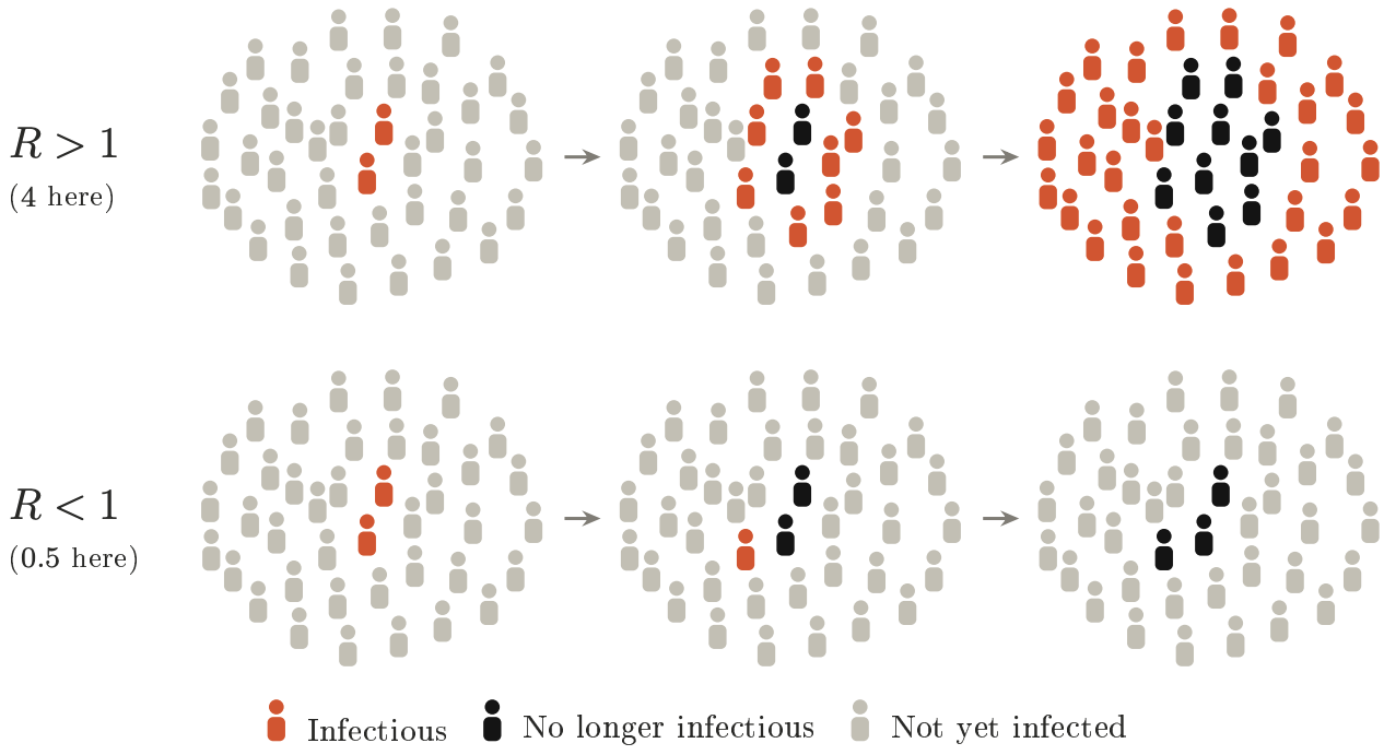
Figure 1. If the reproduction number R>1, the pathogen spreads exponentially. If R<1, spread fizzles out, and the pathogen can be contained.

R depends on the properties of the pathogen, the measures people take to protect themselves, and the population that’s already immune. For a fully susceptible population without interventions, R becomes the basic reproduction number, R₀. For the initial strain of SARS-CoV-2, R₀ was between 1.5 and 6.5. While it’s hard to estimate, smallpox probably had an R₀ of around 3.5 to 6. Measles is commonly cited to have an R₀ of 12-18, although various studies report much larger values.

The aim when fighting a worst-case pathogen is to bring R below 1 for the entire population. If this can be achieved, the disease will not spread, and almost no one will die. This is what we saw with SARS-CoV-1: even though the pathogen was very lethal, we brought the spread down, and so almost no one was infected. SARS-CoV-2, on the other hand, was much less lethal, but we were not able to bring R below 1 consistently, and almost everyone in the world has been infected at some point. Merely slowing the spread of the worst-case pathogen is much less helpful, because of the high mortality rate: spread needs to be stopped outright.

Physical isolation stops all spread, but not everyone can isolate

All pathogens face a fundamental constraint: they must physically enter a human body to cause harm. This gives us a simple way to stop a worst-case pathogen from spreading, at least temporarily. We only need to physically separate all humans (or households) from one another: if the pathogen can’t travel between humans, it can’t spread. For respiratory pathogens, this means making sure isolating households aren’t breathing the same air.

However, separating everyone isn’t possible: some people do work that is essential to keeping society running, and often they need to interact with others. These essential workers maintain the core infrastructure we all depend on, like power plants, industrial supply chains, and medical countermeasure manufacturing. How many essential workers there are varies by country and definition: in the US, estimates range from around 10 to 30 million.

This suggests a “minimum viable path” for protecting society from a worst-case pathogen. As soon as a pathogen is detected, all non-essential workers stay home. Then, we need to stop spread — that is, bring R below 1 — among the essential worker population, so that we can keep essential services running without endangering those workers. This situation needs to be maintained until we can develop longer-term solutions, such as vaccines.

Shutting down all but essential services is very costly, and only makes sense for a pathogen where the consequences of widespread infection are even worse. But faced with something like COVID with a 30% mortality rate, lockdowns seem clearly worth it — and we think most people would choose to stay home anyway. The harder problem would be making sure essential workers feel safe and able to keep working.

A worst-case pathogen is likely respiratory and airborne

A worst-case “wildfire” pathogen, spreading quickly enough to interrupt essential societal functions, is overwhelmingly likely to be respiratory. Respiratory pathogens spread when infected people breathe, sneeze, or cough out infectious particles, and these particles find their way into another human’s respiratory tract. SARS-CoV-2, smallpox, and measles all spread this way. Respiratory pathogens are hard to stop: it’s often much easier to avoid skin-skin contact, contaminated food/water, or insect vectors than it is to avoid breathing the same indoor air.

Infectious particles come in a range of sizes, and size determines how they behave. Larger particles fall to the ground quickly and only infect people at close range (a few meters); smaller ones stay aerosolized and can be inhaled by people much further away. This is often split into “droplet” and “airborne” transmission, but it’s really a spectrum: even relatively large particles can stay airborne for quite some time. The widely used 5 μm threshold between droplets and airborne particles, and the associated droplet-versus-airborne debate you might remember from COVID, were based on a scientific misunderstanding. In reality, there’s nothing particularly special about the cutoff, and all respiratory diseases spread to some extent through both pathways.

Airborne transmission allows for greater spread than droplet transmission, because you share indoor air with far more people than you stand close to. SARS-CoV-2, influenza, rhinovirus, and measles are all substantially airborne (measles can spread between people who weren’t in the room at the same time), and smallpox was likely airborne as well. Blocking airborne transmission is therefore the highest priority for stopping a worst-case pathogen from spreading; if we can manage that, the other transmission pathways are much easier to handle.

We can stop spread among essential workers by preventing exposure to infectious particles

People with respiratory infections emit infectious particles into room air. Most particles are physically removed — for example, they fall to the ground or escape through open windows — or lose their infectivity as the pathogen inside them degrades. But a small fraction of these particles may be inhaled by other people, and this can cause infection.

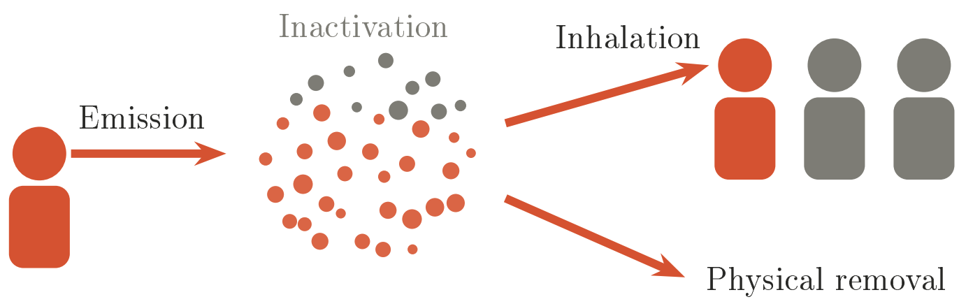
Figure 2. Infected people emit infectious particles into indoor air: if these particles get inhaled by others, they can cause new infections. Only a small fraction of infectious particles get inhaled: most are physically removed, or lose their infectiousness as the pathogen degrades (gray particles).

The reproduction number R, which determines whether the disease can spread, depends on three main factors:

1. How many particles does an infected person exhale?
2. How likely are these particles to get inhaled by others?
3. How likely is an inhaled particle to cause infection?

(1) depends on how abundant the pathogen can get in the respiratory tract, and how long the person remains infectious. (2) depends on how long others spend around the infected person, how many people are in the room, and how much of the room air they breathe in. (3) depends on the pathogen’s specific biology. We model these in more detail in Appendix A, taking into account that particles of different sizes behave differently.

Driving particle exposure to zero would drive R to zero: if nobody breathed in any of the particles, there would be no infections. To stop spread among essential workers, we need to sufficiently reduce their exposure to infectious particles.

Respirators reduce the number of infectious particles you inhale

We can reduce exposure to infectious particles using respirators: devices that fit tightly to the face and filter the air you inhale. Filtering-facepiece respirators (FFRs) are made almost entirely of the filtering material itself, and include the familiar N95, FFP2, or KN95 models. Elastomeric half-mask respirators (EHMRs) consist of a rubber or silicone mask that fits tightly over your nose and mouth, supplemented with replaceable filter cartridges. A full-face respirator is similar, but also covers the eyes, while powered air-purifying respirators (PAPRs) use a fan to blow filtered air into a mask or hood. Elastomerics and PAPRs are commonly used by industrial workers, for example to avoid breathing in lead dust.

Not every mask is a respirator. Surgical masks fit loosely and let past a lot of air, making them bad at filtering the air you inhale. They were designed to stop large particles, like the surgeon’s saliva, from falling into a patient’s open wound during surgery. They were never meant to provide respiratory protection, nor are they particularly effective at this task, despite their widespread use during the COVID pandemic.

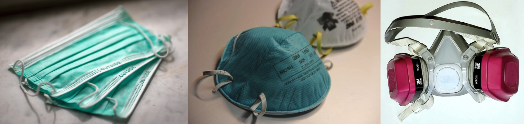
Figure 3. From left to right: surgical masks, an N95 filtering-facepiece respirator (FFR), and an elastomeric half-mask respirator (EHMR). (Image sources: here, here, and here.)

Respirators can be very effective at stopping infectious particles from being inhaled. Respirator efficiency is measured by the protection factor (PF): a protection factor of 10 lets through only 1/10th of all airborne particles. An N95 respirator is designed to filter out at least 95% of particles: if it fit perfectly to the face without leaks, it’d have a PF of at least 20. EHMRs with P100 filters are designed to filter out at least 99.97% of particles, so a perfectly-fitting EHMR would have a PF larger than 3000. Filters are usually tested at the most penetrating particle size, and so their averaged performance across all particle sizes is often substantially better than the rated value implies.

In practice, protection factors are limited by how well the respirator fits the face. If some fraction \(f\) of inhaled air slips through a gap in the face-seal, it won’t pass through the filter, and the maximum achievable protection factor will be \(1/f\).¹ The respirator also needs to be worn consistently: if it’s removed a fraction\(\ f\) of the time, the maximum achievable protection factor is also \(1/f\). Fit can be improved through training, and by having people do a fit test. Fit can be tested using particle counters, or by spraying bitter or sweet substances at the user and seeing whether they can taste them through the respirator.

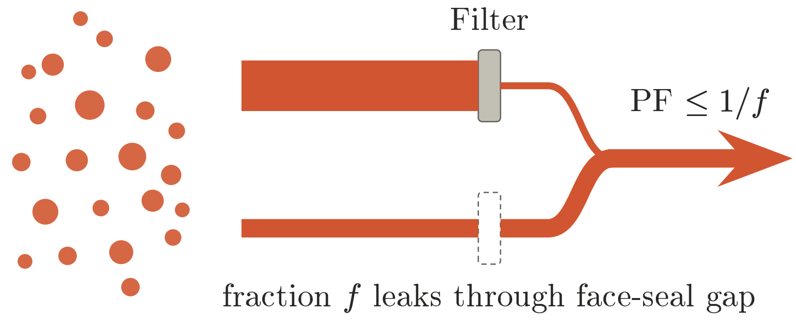
Figure 4. Respirator filters effectively block particles, reducing how many particles get inhaled. But if some fraction \(f\) of inhaled air leaks past the filter, at least \(f\) of all particles are guaranteed to make it through. The respirator’s protection factor (PF) can therefore be no higher than \(1/f\). A similar effect applies if the respirator is removed a fraction \(f\) of the time.

For any given respirator, the “assigned protection factor” (APF) sometimes provided by regulatory bodies is not the same as the “real” protection factor achievable in practice. The real protection factor is an empirical quantity — how well the respirator actually filters air — and varies for different faces and usage patterns. The APF is used to make sure workers in a given environment are always sufficiently protected, and is thus usually a deliberate underestimate, more akin to a realistic worst case.

Respirators also block exhaled particles, greatly increasing their effectiveness

A well-fitting respirator that filters air in both directions also stops infectious particles from being exhaled. This is known as “source control”. Not all respirators have source control: some have exhalation valves, which let air exit without filtering it. However, most FFRs and some EHMRs come without exhalation valves, and some manufacturers sell filters that can be attached to the exhalation valve to restore source control.

If the respirator filters exhaled air as well as inhaled air, the protection factor acts twice to reduce everyone’s exposure. The number of infectious particles exhaled into the room is divided by PF, and the number of particles anyone inhales from room air is also divided by PF. The total reduction in exposure is PF².

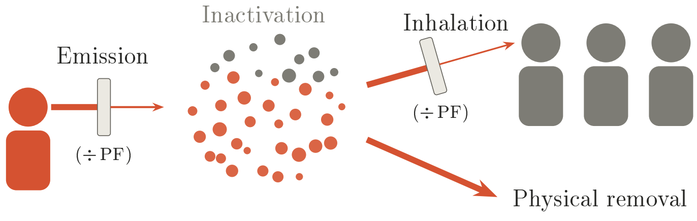
Figure 5. If everyone wears respirators (with “source control”), infected people emit fewer particles into the room, and others inhale fewer particles from room air. Both emission and inhalation are reduced by a factor of PF, yielding a net exposure reduction of PF².

Appendix B discusses observed protection factors for FFRs and EHMRs, and some nuances for calculating the average “group” protection factor. In short, N95-type FFRs can probably achieve group PFs of 15-40, and EHMRs can achieve PFs ranging from 30 well into the hundreds. The upper ends of both ranges are achieved via fit testing, and potentially by removing individuals who fail a fit test. To summarize:

Respirator	Filter efficiency	Achievable group protection factor
N95-type filtering-facepiece (FFR)	At least 95%, i.e. less than 1 in 20 particles pass through	15 to 40
Elastomeric half-mask (EHMR), with P100 filter	At least 99.97%, i.e. less than 1 in 3000 particles pass through	30 to 100+?

Beyond inhalation, some respiratory pathogens can also infect you if you touch a fomite (contaminated surface) and then touch your eyes, nose, or mouth. Respirators also effectively block fomite transmission. They both reduce the number of particles that settle onto surfaces in the first place, and physically stop people touching their nose and mouth. That leaves the moments when a respirator comes off — using the bathroom, or taking a break — but handwashing, hand sanitizer, and surface cleaning handle fomite transmission well in those cases.

Respirators drive R below 1 for even a worst-case pathogen

We haven’t seen a worst-case pathogen before, and so it’s hard to know how transmissible it might be. But stopping spread among essential workers only requires stopping transmission between people still well enough to be at work. Someone coughing up their lungs in a hospital bed isn’t the case we’re worried about — they’re obviously sick, and would be isolating rather than out running society. The case that matters is the worker who feels fine, or nearly so, and spreads the pathogen without knowing it.

For that case, even a worst-case pathogen is fairly constrained. It can make you cough and sneeze more, and raise the concentration of infectious particles you emit — but those symptoms are conspicuous, and anyone showing them would be staying home. Among workers who are out and breathing and talking roughly normally, even a worst-case pathogen isn’t dramatically changing how much they emit. No pathogen can defend against gravity or ventilation either, and once inhaled it can only be so infectious.

Assuming that essential workers stay at home if strongly symptomatic, we calculate (Appendix A) that respirators with a group protection factor of about 18 are sufficient to stop a pathogen as transmissible as measles. Measles is extremely transmissible — compare the widely cited R₀ of 12-18 to the initial SARS-CoV-2 R₀ of 1.5-6.5 — and we think that a highly lethal pathogen as transmissible as measles is a plausible worst case. Real-world achievable protection factors (see above) seem straightforwardly sufficient to stop this.

Moving beyond anything resembling existing pathogens, Appendix A also considers more extreme theoretical upper bounds on transmissibility. Even under these bounds, we think that respirators with protection factors ranging from 30 to 60 should be sufficient to stop the pathogen from spreading. It’s not entirely clear what group protection factors are achievable at large-scale among previously untrained workers, but even a group protection factor of 60 is not obviously out of the reach of EHMRs. We think it’s very unlikely that a pathogen necessitating respirators with PF 60 is biologically feasible.

These results also imply that respirators with protection factors lower than 18 could have stopped SARS-CoV-2, if everyone had worn them consistently around others. That might sound surprising given how much masking happened during COVID, but a respirator only protects you while you wear it. COVID masking was partial and inconsistent, and mostly involved loose surgical masks that were frequently removed. Against a far more lethal pathogen, we expect essential workers to feel a much stronger desire to protect themselves, their coworkers, and their families.

Respirators are cheap, and can be stockpiled

A single FFR costs around $1 at bulk prices and lasts maybe a few days before the straps break or the fit significantly degrades. A single EHMR costs around $30 at bulk prices, and can be reused for years. If respirators need to be worn for more than ~3 months, EHMRs are cheaper (on top of being more protective). Considering these and other stylized numbers:

Respirator type	Unit cost (bulk)	Lifetime	Cost per person per day (1 year)
Filtering facepiece (FFR)	$1	~3 days	$0.33
Elastomeric half-mask (EHMR)	$30	Years	$0.08
Elastomeric full-face	$150	Years	$0.40
Powered air-purifying (PAPR)	$1000	Years	$2.73

Elastomeric full-face respirators can provide somewhat larger protection than half-masks, but can cost 5 times as much. Powered air-purifying respirators can yield real-world protection factors in the thousands or higher, but are much more expensive, need continuous battery power, and often don’t have source control. At current prices, we think that EHMRs occupy the “sweet spot” for large-scale stockpiling: they are cheap enough that they can be bought in large quantities, and are probably sufficient to stop any pathogen if worn universally.

The cost of stockpiling EHMRs for essential workers is basically a rounding error compared to other government expenditures. To take the US as an example, buying 20 million EHMRs for essential workers would cost around $600 million; even if storing and distributing them costs another $600 million, a 20-year stockpile would cost on average $60mn/year, less than 0.001% of federal government spending. Protecting essential workers in many other countries would be similarly cheap.

Other interventions complement respirators, but can’t substitute for them

Beyond respirators, there are many other ways to reduce infectious particle exposure. We could physically remove particles from the air faster, using air filters (e.g. Corsi-Rosenthal boxes), and better ventilation. We can inactivate the infectious particles without removing them, using far-UVC light, or glycol vapors at low concentrations. Collectively, we can refer to these interventions as “indoor air cleaning”.

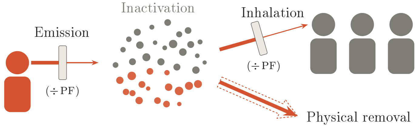
Figure 6. Improved ventilation/air filtration removes more particles from the air (dashed arrow); far-UVC or glycol vapors inactivates them where they are (gray particles).

Unfortunately, indoor air cleaning is not nearly as powerful as respirators: see Appendix C for more details. If everyone in a room wears respirators with PF 30, the number of inhaled infectious particles is reduced by a factor of 900. Realistic increases in ventilation and air filtration for typical workplaces are at most equivalent to a 5x reduction in inhaled infectious particles. Peak achievable far-UVC or glycol deployments are comparable to exposure reductions in the multiple tens. None of these interventions — or even indoor air cleaning as a whole — can substitute for respirators: the PF² effect makes respirators unreasonably effective.

Diagnostics, like the rapid tests used to detect SARS-CoV-2, can help make sure even asymptomatic workers stay at home. Again, this would reduce R, but can’t substitute for respirators. Unlike indoor air cleaning, we can’t prepare diagnostics ahead of time: we need to know what the pathogen is first.

Even though they can’t substitute for respirators, these interventions are still extremely valuable! Suppose a pathogen does emerge that demands a respirator PF of 30: in other words, we need to reduce infectious particle exposure by \(30^2 = 900\). If other interventions can provide a 4x reduction, the required respirator PF is only \(\sqrt{900/4}=15\). This is a much lighter lift, and reduces the level of respirator fit that’s required to stop spread. All of these interventions have a role to play, but respirators are the backbone on which everything else must build.

Appendix A: Upper bounding disease spread among essential workers

A.1 We can upper-bound \(R_0\) using the “infection rate” \(\Phi\)

While \(R_0\) is hard to calculate from first principles, we can upper-bound it using an instantaneous infection rate for indoor spaces, \(\Phi\), which is the rate at which one infected person infects others when everyone nearby is susceptible. If \(\Phi\) equals 1 infection/hour, on average 1 person in that room could get infected every hour.

Any given infection event is random and independent. As a result, the probability that everyone in a room remains uninfected over a time period \(T\) is just \(e^{-T\Phi}\), which follows from the Poisson statistics of random independent events and matches the classic Wells–Riley picture of airborne transmission. The chance that at least one new infection has occurred is therefore \(1-e^{-T\Phi}\), and on expectation at most \(T\Phi\) new infections have occurred.

Assume that the infected person spends a time \(\tau_W\) infectious and among others, and that the infection rate \(\Phi\) is constant across this time period. Then, the number of people they’ve infected is at most² the infection rate multiplied by this time period:

\[R_0 \;\le\; \Phi\,\tau_W .\]

Pathogen concentrations in respiratory fluid vary by orders of magnitude throughout the course of infection, and so \(\Phi\) should vary by orders of magnitude as well. To upper-bound \(R_0\), we’ll assume that \(\Phi\) is always equal to the peak infection rate.

We set \(\tau_W\) to 50 hours, equal to an extended week-long shift. While the total time a worker spends infectious could be longer, if \(\Phi\) varies by orders of magnitude throughout infection, \(R_0\) will be dominated by the period of peak infection. \(\tau_W=50\) hours is a reasonably conservative estimate for the length of this period: it assumes a worker remains at peak infectivity for an entire week.

A.2 Calculating the infection rate

Exhaled aerosol particles range from around \(0.1\) to \(100\ \mu\text{m}\) in diameter. For particles with diameter \(D\), the infection rate \(\Phi\) is the product of the following terms:

1. The rate \(\varepsilon(D)\) at which aerosols are emitted by the infected person
2. The probability \(\alpha(D)\) that an aerosol is inhaled by a susceptible person
3. The probability \(\varsigma(D)\) that an inhaled aerosol causes infection

We can calculate the total infection rate \(\Phi\) by integrating (i.e summing) this product across all diameters:

\[\Phi = \int dD\; \varepsilon(D)\,\alpha(D)\,\varsigma(D).\]

Each of these three terms gets its own subsection: \(\varepsilon(D)\) is discussed in A.3, \(\alpha(D)\) in A.4, and \(\varsigma(D)\) in A.5. A.6 discusses maximum “quanta concentrations”: how infectious a pathogen can be once inhaled. A.7 summarises the results.

Our model is structurally similar to existing state-of-the-art models for respiratory disease transmission. One difference is that we resolve the full distribution of aerosol sizes, tracking how emission, airborne lifetime, inhalation, and infectivity each depend on particle diameter. The more important difference is our aim: rather than attempting to realistically model any specific disease, such as COVID-19, we want worst-case bounds on transmission. We therefore make some simplifying assumptions that deliberately overestimate transmission where useful.

A.3 Aerosol emission rate, \(\varepsilon(D)\)

We calculate the emission rate \(\varepsilon(D)\) by multiplying measured number concentrations \(n(D)\) of exhaled aerosol per unit volume of air, for various activities, with estimates of how much air people expel during those activities. Activity-specific inhalation rates (\(\approx\) exhalation rates) come from the EPA Exposure Factors Handbook (2011); for context, a typical daily mean is 0.67 \(m^3\)/hr.

Speech and coughing move additional air. Following Pöhlker et al. (2023), we assume that a person expels 540 L/hr during normal speech and 1080 L/hr when louder, that a person exhales 1.5 L per cough, and that a normal person will cough around once per hour.

Finally, we need the fraction of time a human spends in these different aerosol production modes, which depends on the context they’re in. There aren’t standard parameters for this, so we come up with our own:

Scenario	Sleep	Light	Moderate	Heavy	Speak (normal)	Speak (loud)	Coughs/hr
Sleeping	1.0	—	—	—	—	—	—
Daily	0.40	0.35	0.10	0.02	0.10	0.03	1
Office	—	0.70	0.10	—	0.15	0.05	1
Manufacturing	—	0.40	0.35	0.10	0.05	0.10	1

Coughing increases the number of aerosol particles in a given volume of exhaled air, and heavy coughing also increases the overall airflow. Someone coughing 100 times per hour releases around 10x the particles of a non-cougher. But we assume that someone this symptomatic will stay at home, either voluntarily or because society/their workplace requires it.

A.4 Inhaled fraction, \(\alpha(D)\)

We assume that the air in the room is well-mixed, so that a given aerosol particle is equally likely to be inhaled by anyone. This forms the basis of the classic Wells-Riley approach, and is generally well justified by the physics of air motion.³

In a room of volume \(V\), the equilibrium particle concentration

\[C_\text{eq}(D) = \frac{\varepsilon(D)\,\tau_A(D)}{V},\]

where \(\tau_A(D)\) is the mean airborne lifetime of an aerosol with diameter \(D\). If \(N\) susceptible people each breathe at rate \(\dot V_E\), the fraction of emitted aerosols they inhale is

\[\alpha(D) = \nu_I\,\tau_A(D), \qquad \nu_I = \frac{N\,\dot V_E}{V},\]

where \(\nu_I\) is the rate at which the room’s air is inhaled by susceptible people. We take \(\dot V_E\) as 0.72 \(\text{m}^3/\text{hr}\), the EPA “Light Intensity” value, which lets us calculate \(\nu_I\) for any room if we know \(N/V\).

Infectious aerosols leave indoor air by several independent routes: ventilation carries them outside, air filtration removes them from the air, gravity settles them onto surfaces, and the pathogen itself can die (we call this “intrinsic decay”). Each acts at its own rate, such that the overall removal rate \(\Lambda\) is given by

\[\Lambda = \lambda_\text{vent} + \lambda_\text{settling} + \lambda_\text{decay} + \dots, \text{with } \tau_A = \frac{1}{\Lambda}.\]

It’s convenient to consider ventilation and filtration as part of the same term, \(\lambda_\text{vent}\).

Any single \(\lambda_i\) is a lower bound on \(\Lambda\), and so is the sum of any subset of the \(\lambda_i\). And any lower bound on \(\Lambda\) will turn out to give an upper bound on \(\tau_A\) and thus \(\alpha\). For convenience, we therefore only consider ventilation and settling.

\(\lambda_\text{vent}\) is fairly well-studied: it ranges from 0.2-3 \(\text{hr}^{-1}\) in typical buildings, and is usually larger in commercial buildings than in residences. Since, from the above, \(\alpha(D) < \frac{\nu_I}{\lambda_i}\), we can upper bound \(\alpha(D)\) for various locations using \(\lambda_\text{vent}\) alone. Estimating plausible parameters for a range of settings, we find:

Setting	Height (m)	Area/person \((\text{m}^2)\)	\(\lambda_\text{vent}\) \((\text{hr}^{-1})\)	\(\nu_I\) \((\times 10^{-3} \text{ hr}^{-1})\)	\(\alpha_\text{air}\) upper bound (%)
Home	2.5	80	0.35	3.6	1.0
Lecture theatre	6	0.62	4	390	8.8
Office	3	30	1.1	8.0	0.72
Dense office	3	15	1.1	16	1.4
Light assembly	6	20	5	6.0	0.12
Heavy assembly	6	40	10	3.0	0.03
Warehouse	6	200	0.2	0.6	0.30

We can sense-check these results using indoor \(\text{CO}_2\) concentrations. Ambient outdoor \(\text{CO}_2\) concentrations are around 400 ppm (parts per million), while the \(\text{CO}_2\) concentration in exhaled breath is much higher, around 30000 ppm. If offices are kept below 1000 ppm (a common recommendation), then \(\alpha\) is likely no higher than (1000-400)/30000 = 2%, consistent with the above estimates.

To a good approximation, \(\lambda_\text{settling}\) depends only on the (downward) speed \(v_s\) at which the aerosols settle, such that

\[\lambda_\text{settling}(D) = \frac{v_s(D)}{H},\]

where \(H\) is the height of the room. We determine \(v_s\) using Stokes’ law, with additional corrections at small and large particle diameters.⁴

Finally, aerosolized pathogens also become inactivated over time. Published half-lives for various pathogens in aerosol range from minutes to many hours. In the absence of UV, SARS CoV-2 appears to have a half-life of around 1 hour, corresponding to a decay rate \(\lambda_{\text{decay}}\) of 0.7/hr.

Since there’s a lot of variation in decay rates for different pathogens, we neglect \(\lambda_{\text{decay}}\) and take \(\Lambda=\lambda_\text{vent} + \lambda_\text{settling}\). This is a lower bound that tends to overestimate lifetimes and thus transmission.

A.5 Infection probability, \(\varsigma\)(D)

Infection probability \(\varsigma(D)\) is the product of two factors: the probability an inhaled particle deposits on respiratory tract tissue, and the probability a deposited particle causes infection. We derive the former using the ICRP model of particle deposition in the respiratory tract, which is widely used in infection modeling, and the latter by assuming a certain quanta concentration \(c_q\) per mL of aerosol fluid.

Each aerosol particle exhaled by the infected person will carry some number of infectious quanta. If \(q\) quanta are deposited in a susceptible person’s respiratory tract,⁵ the total infection probability is

\[P(\text{infected}) = 1-e^{-q}.\]

A single quantum is the dose of pathogen which leads to a \(1-e^{-1}\approx63\%\) chance of infection. Unlike infection probabilities, quanta add linearly: exposure to \(q_1\) quanta followed by \(q_2\) quanta is the same as exposure to \(q_1+q_2\) quanta.

Define the quanta concentration \(c_q\) as the number of quanta per mL of aerosol fluid. Then, the total number of quanta in an aerosol particle of initial diameter⁶ \(D_i\) is

\[q(D_i) = \frac{\pi}{6} D_i^3\, c_q,\]

and the infection probability, conditional on deposition, is:

\[P(\text{infection}\mid\text{deposition}) = 1 - e^{-q(D_i)} = 1 - e^{-\frac{\pi}{6} D_i^3 c_q}.\]

The fact that quanta per aerosol scale as \(D_i^3\) tends to make larger particles much more infectious than smaller particles. However, larger particles also settle faster, and thus exit room air more quickly.

The quanta concentration \(c_q\) is set by the concentration of pathogens in respiratory tract fluid, and thus varies hugely throughout the course of infection. For simplicity, and to remain conservative, we assume that \(c_q\) sits at its maximum value (see the next section), for the entire duration \(\tau_W\).

A.6 Maximum quanta concentrations

The quanta concentration \(c_q\) depends on (1) the pathogen concentration per unit volume of released aerosol particles (“viral load”, or “bacterial load”), and (2) the number of quanta per unit of pathogen.

A.6.1 Maximum viral loads observed in nature

Viral loads can be measured using swabs, or directly in sputum, the fluid that’s actually coughed out. Neither corresponds exactly to the viral loads in aerosol fluid, but we’ll assume they are reasonable approximations. Common measurement units include \(\text{TCID}_{50}\) (median tissue culture infectious dose), PFU (plaque-forming unit), and FFU (focus-forming unit): these are all roughly equivalent to 1 “infectious unit” in cell culture.⁷ Counts of viral RNA copies in a sample are much higher: for SARS CoV-2 and influenza-like viruses there are around \(10^4\) RNA copies per infectious unit.⁸

Viral loads vary by orders of magnitude over the course of an infection, and also vary significantly between viruses, patients, and locations in the respiratory tract. Our goal here is to estimate the peak viral load an infection can reach: we will assume this load is maintained for the entire period \(\tau_W\).

Mikszewski et al. (2022), drawing on other studies, give \(\log_{10}\) mean and standard deviation viral loads for a number of viruses.⁹ From these, we take an approximate “peak” value as being two \(\log_{10}\) standard deviations above the mean;¹⁰ where results were in RNA copies/mL, we convert peak values to \(\text{TCID}_{50}\) using the \(10^4\):1 ratio described above. (This yields maximum values broadly consistent with other measurements.)

Virus (data source)	log\(_{10}\) mean \(\pm\) st. dev	“Peak” value
Adenovirus (swab)	3.2 \(\pm\) 0.95 \(\text{TCID}_{50}\)/mL	\(10^{5.1}\) \(\text{TCID}_{50}\)/mL
Coxsackievirus (swab)	3.4 \(\pm\) 1.1 \(\text{TCID}_{50}\)/mL	\(10^{5.6}\) \(\text{TCID}_{50}\)/mL
Measles (swab)	3.5 \(\pm\) 1.6 \(\text{TCID}_{50}\)/mL	\(10^{6.7}\) \(\text{TCID}_{50}\)/mL
Rhinovirus (swab)	3.6 \(\pm\) 0.83 \(\text{TCID}_{50}\)/mL	\(10^{5.26}\) \(\text{TCID}_{50}\)/mL
Influenza (sputum)	6.7 \(\pm\) 0.84 RNA copies/mL	\(10^{4.38}\) \(\text{TCID}_{50}\)/mL
MERS (sputum)	6.7 \(\pm\) 1.6 RNA copies/mL	\(10^{5.9}\) \(\text{TCID}_{50}\)/mL
SARS-CoV-1 (sputum)	6.1 \(\pm\) 1.3 RNA copies/mL	\(10^{4.7}\) \(\text{TCID}_{50}\)/mL
SARS-CoV-2 (sputum)	5.6 \(\pm\) 1.2 RNA copies/mL	\(10^{4}\) \(\text{TCID}_{50}\)/mL

Based on this, we estimate that \(10^7\) \(\text{TCID}_{50}\)/mL is a realistic upper bound for real-world peak viral loads. The pathogen that comes closest to reaching it is measles, with a 97.5th percentile of \(10^{6.7}\) \(\text{TCID}_{50}\)/mL.

A.6.2 Upper bounds for any virus

Viral loads for any virus must eventually hit a ceiling. As the absolute hard limit, there can be no more viruses within 1 mL of respiratory fluid than could physically fit inside that 1 mL. A SARS CoV-2 or influenza-like virus might be spherical, be around 100 nm wide, and have \(10^4\) virions per \(\text{TCID}_{50}\). This implies that there can physically be no more than around \(10^{11}\) \(\text{TCID}_{50}\) in 1 mL of space. (This number doesn’t generalize across all viruses: some are smaller, and the ratio of virions to infectious units might vary.)

More realistic upper bounds come from biology. There are only around \(10^{11}\) lung epithelial cells that are realistic targets for a respiratory virus, the turnover rate of these cells is at most \(3 \times 10^8\) cells/day, an infected cell probably generates around 10-100 infectious viral units,¹¹ and the respiratory tract probably generates at least 100 mL of fluid per day.¹²

Suppose all \(10^{11}\) lung epithelial cells were infected and killed over the course of 1 day, each producing 100 infectious units, and those units were spread equally through 100 mL of fluid and exhaled. The total concentration could then be at most \(10^{11}\) \(\text{TCID}_{50}\)/mL. (Note these are extremely conservative estimates.) If only 10% of the lung epithelial cells could realistically be infected in 1 day, each producing only 10 infectious units, the viral load falls to \(10^{9}\) \(\text{TCID}_{50}\)/mL.

Symptoms should arise at the very latest once cells are being infected as fast as they turn over (upper bounded at 3\(\times 10^8\) cells/day). At 100 infectious units/cell spread over 100 mL of fluid, the maximum viral load while asymptomatic is \(3\times 10^8\) \(\text{TCID}_{50}\)/mL.

Even this tissue-damage bound is still deliberately conservative. In reality, both symptoms and the immune control that eventually caps infections are driven by immune activation, which sets in well before acute tissue damage. We use the more conservative tissue-damage bound because immune dynamics are much harder to model and more pathogen-dependent. Because immune activation dominates in practice, observed viral loads are orders of magnitude below this bound.

Based on the above we think that \(10^{10}\) \(\text{TCID}_{50}\)/mL is a strong upper bound on viral loads for any possible respiratory virus, and that the true upper limit, especially while asymptomatic, is orders of magnitude lower.

A.6.3 Maximum quanta per virion

How many infectious quanta are there per \(\text{TCID}_{50}\)? Infecting an optimized tissue culture should be easier for a virus than infecting a human body, so we should generally expect \(\lesssim\) 1 quantum per \(\text{TCID}_{50}\). Measles likely comes close to this bound,¹³ while for SARS CoV-2 the ratio is smaller, around 0.075.¹⁴

All things considered, this suggests the peak quanta concentration \(c_q\leq10^7\) quanta/mL for any observed respiratory virus. Measles, one of the most transmissible pathogens known, is the example that most clearly reaches this bound.

We think it’s unlikely there could be a respiratory pathogen significantly more transmissible than measles. An extreme theoretical upper bound is \(c_q\leq10^{10}\) quanta/mL, but we think the true upper limit, especially while asymptomatic, is likely orders of magnitude below this.

A.6.4 Bacteria

Bacterial loads must also eventually hit a ceiling. At most \(10^{13}\) bacteria could physically fit into a 1 mL volume;¹⁵ as before, this is an extreme upper bound and many orders of magnitude above maximum measured concentrations. Total bacterial concentrations in the healthy human respiratory tract are as high as \(10^8\) 16S rDNA copies/mL, and it seems unlikely that a bacterial pathogen could significantly exceed this while the person remains asymptomatic.

Mikszewski et al. (2022) estimate that peak bacterial load in untreated tuberculosis infections reached \(5.5 \pm 1.3 \log_{10}\) CFU/mL, suggesting a 97.5th percentile maximum of \(10^{8.1}\) CFU/mL. (A colony-forming unit is the dose which can establish a colony in nutrient culture.)

Infectious doses (i.e., quanta/bacterium) vary hugely. For example, when 17 cynomolgus macaques were bronchoscopically inoculated with 25 CFU of tuberculosis, all of them were infected, suggesting there are perhaps 0.1 quanta/CFU. By contrast, in human challenge trials for Streptococcus Pneumoniae, colonization occurred in 30% of subjects at a dose of \(10^4\) CFU, and 60% of subjects at a dose of \(10^5\) CFU.

Taken at face value, these results suggest that tuberculosis might reach \(10^7\) quanta/mL. But this seems somewhat implausible: it matches the peak quanta/mL for measles, which has much higher \(R_0\) than tuberculosis.

Theoretically, we should expect \(\leq\) 1 quantum/CFU, similar to viruses. The observed numbers seem consistent with this bound, and are often much below it.

Overall, we estimate that \(c_q \leq 10^{7}\) quanta/mL for all extant bacterial respiratory pathogens. It seems unlikely that a bacterial pathogen could exceed \(10^8\)-\(10^{9}\) quanta/mL, especially while the infected person remains asymptomatic.

A.7 What respirator protection factors can stop spread?

Our model outputs upper bound infection rates in different settings, as a function of peak quanta concentration \(c_q\). This gives the below result:

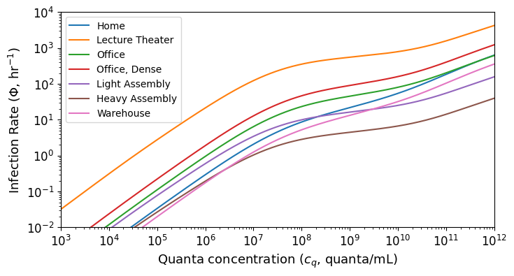
Office infection rates are themselves an upper bound on the infection rate in most settings (except in the lecture theatre).

Any intervention that reduces the exposure to infectious particles (i.e. \(\alpha(D)\)) by some factor also reduces \(\Phi\) by the same factor.

Since \(R_0\leq\Phi \tau_W\), reducing the infection rate by just over \(\Phi \tau_W\) guarantees that \(R<1\) and that spread stops. If everyone wears respirators, the required group protection factor to achieve this is \(\sqrt{\Phi \tau_W}\).

Specializing to the office setting, we find:

Quanta concentration \((c_q, \text{quanta/mL})\)	Infection rate \((\Phi, \text{hr}^{-1})\)	Required infection rate reduction \((\Phi\tau_W)\)	Required respirator PF (rounded up)
\(10^7\)	6.4	320	18
\(10^8\)	23.4	1170	35
\(10^9\)	45.5	2275	48
\(10^{10}\)	60.5	4025	64

As discussed in A.6, \(10^7\) quanta/mL is likely a realistic upper limit. This corresponds to a protection factor of 18. Protection factors in the range 30-65 are sufficient to stop spread up to the extreme theoretical upper limit.

Appendix B: Achievable “group” respirator protection factors

B.1 The group protection factor is not the mean protection factor

Respirators will fit different people’s faces more or less well. Different people wearing the same respirator will therefore have different protection factors. What is the relevant “group” protection factor across all the people in the room?

Assume we have N people in a well-mixed room, each of which is wearing a respirator with some PF. Some of these people are infected, but we don’t know who, and the PFs are heterogeneously distributed. The rate at which people exhale infectious particles into room air is reduced by the mean value of \(1/PF\), and so is the rate at which people inhale particles from the room. The relevant “group” PF — which describes the total exposure reduction — is therefore the harmonic mean (HM). The harmonic mean is 1 divided by the mean value of 1/PF. It differs from the “standard” arithmetic mean, which is just the mean value of PF.¹⁶

To complicate things further, studies of respirator performance usually report the geometric mean (GM) and geometric standard deviation (GSD). These are natural statistics to use when your data varies across orders of magnitude, and/or is lognormally distributed, which measured protection factors often are. For lognormal distributions, the HM is \(\text{GM} \times \exp(-\ln(\text{GSD})^2/2)\).

B.2 Experimental results

Many studies have measured FFR and EHMR protection factors. There are two particularly relevant quantities:

• Workplace protection factor (WPF): the “true” protection factor for inhalation, during the relevant workplace activity, averaged over all the time the activity takes place. This is hard to measure, and is rarely measured directly.
• Simulated workplace protection factor (SWPF): the measured protection factor for inhalation during some shorter period (e.g. 10 minutes) in which the participant is asked to simulate various workplace movements, e.g. walking, turning the head, bending over, and so on.

Lee et al. (2016) measured SWPF for 30 participants for various respirators; the participants were trained and fit tested before the start of the experiment. On average, they found that FFP2 respirators had GM SWPFs of 27.1, with a GSD of 2.7, and a 5th percentile value of 6.7. The GM went up to 30.9 for participants that passed a fit test. An earlier study by Lawrence et al. (2006) found an average GM of 20.4 and GSD of 3.1 without fit testing, although the GM could go as high as 55.0 depending on the model.

Perhaps the academic study that has come the closest to measuring true WPF for FFRs is Duncan et al. (2020). Here, seven subjects wore an N95 FFR for most of the workday for 5 consecutive days, and performed 30-minute SWPF tests every other day. The subjects were all trained in how to wear a respirator, and quantitatively fit tested before the start of the experiment. The combined GM SWPF across all the measurements was 43, with a geometric standard deviation of 1.4.

Elastomeric half-mask respirators not only have much better filtration, but also much better fits. For an EHMR with only an N95 filter, GM SWPF in the Lawrence et al. experiments went up to from 20 to 35.5 compared to the N95 FFRs, and this must be due to fit rather than filter. For EHMRs with P100 filters, Janssen and McCullough (2009) measured cumulative WPFs during long (>2 hour) tasks in a lead battery plant among workers who were both trained in respirator use and fit tested, and found a median (\(\approx\) GM) of 270, with a 5th percentile at 53 (implying a GSD of about 2.23). Vo et al (2015) studied SWPF against nanoparticles; while the sizes are a little different than typical respiratory aerosols, results from the most relevant regime (100-400nm) had a GM of 6780, with a 5th percentile of 1199 (implying a GSD of around 2.37).

As discussed above in B.1, group protection is best described using the harmonic mean (HM) rather than the geometric mean (GM). Summarizing some of the most relevant studies above:

Study	GM (GSD)	HM (inferred)
Lee et al. (2016), FFP2, SWPF, no fit test	27.1 (2.7)	16.5
Lee et al. (2016), FFP2, SWPF, fit test	30.9 (2.5)	20.3
Duncan et al. (2020), N95 FFR, involved 5-day SWPF, fit test	43 (1.4)	40.6
Janssen and McCullough (2009), EHMR with P100 filter, multi-hour WPF, fit test	270 (2.3)	190.86
Vo et al (2015), EHMR with P100 filter, SWPF, fit test	6780 (2.37)	4671.5

While encouraging, none of these studies measure a full-day WPF in a previously untrained population. Early unpublished results by Amodo Design suggest that, for EHMRs, a group of people without prior experience can achieve full-day HM WPFs of around 30. Removing participants who fail a 3.5 min fit test yielded HM WPFs of around 70.

With sufficient training and real incentives to preserve good fit (you don’t want to catch the disease!), we think much larger EHMR WPFs should be achievable, comparable to the results from the earlier workplace studies. If there were cheaply scalable ways to check respirator fit, this could also help a lot.

Appendix C: Indoor air cleaning

Respirators with PF 30 can reduce exposure to infectious particles by \(30^2=900\). They can therefore reduce the infection rate \(\Phi\) by the same amount. How does this compare to indoor air cleaning interventions, like improved ventilation and air filtration, far-UVC, or glycol vapors?

From A.4, the total rate \(\Lambda\) at which infectious pathogen is removed from indoor air is given by

\[\Lambda = \lambda_\text{vent} + \lambda_\text{settling} + \lambda_\text{decay} + \dots.\]

Also, the fraction of emitted infectious aerosols that get inhaled, \(\alpha(D)\), is proportional to \(1/\Lambda\). Therefore, if we make some change to \(\Lambda\):

\[\frac{\alpha_{\text{new}}}{\alpha_{\text{old}}} = \frac{\Lambda_{\text{old}}}{\Lambda_{\text{new}}}=\frac{\lambda_\text{vent, old} + \lambda_\text{settling, old} + \lambda_\text{decay, old} + \dots}{\lambda_\text{vent, new} + \lambda_\text{settling, new} + \lambda_\text{decay, new} + \dots}.\]

If we increase one of the terms in the denominator, say by some factor \(F\), we decrease \(\alpha(D)\) by at most the same factor \(F\).

This already suggests that reducing \(\alpha(D)\) by 900x, comparable to respirators, requires increasing \(\lambda_{\text{vent}}\) by at least 900. Since current ventilation rates are on the order of 1 air change per hour (1 ACH), this implies we need at least 900 ACH, so 1 air change every 4 seconds. This is clearly infeasible: even hospital operating rooms have only tens of ACH. Semiconductor fabrication cleanrooms can achieve hundreds of ACH, but this is expensive and requires purpose-built specialist facilities.

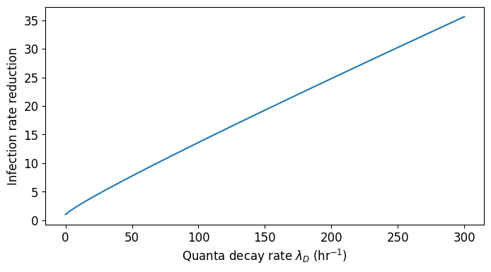
In practice, because of the other terms, this gets even worse. Using our full model to calculate the infection rate reductions from increased \(\lambda_{\text{vent}}\), for \(c_q=10^7 \text{ quanta/mL}\), we find that even an air cleaning rate of 600/hr (600 ACH) only reduces infection rate by 100, way below what respirators can achieve.

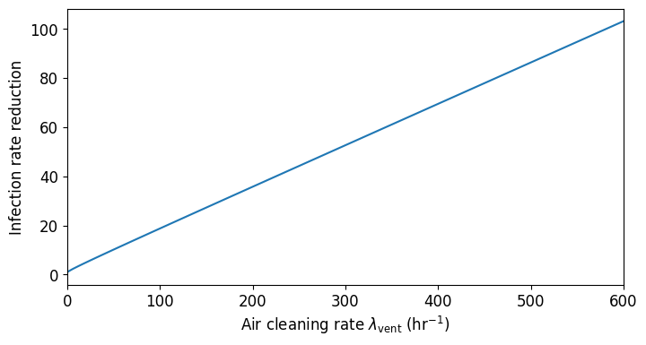
For far-UVC, we can consider estimates of effective air changes per hour (eACH). While data is limited, and there’s variation depending on room geometry and the specific pathogen, the safety-limited eACH ceiling is probably in the tens to low hundreds. From the above figure, this means we should expect infection rate reductions in the low tens, say around 20-40.

We can also directly quantify efficacy using inactivation rates. A dose \(D\) of far-UVC should reduce viable pathogen concentrations (i.e. infectious quanta) according to \(e^{-kD}\), where \(k\) is the susceptibility constant. \(k\) is probably in the range 1.5-15 cm\(^2\)/mJ for coronaviruses, and the 8-hour safe eye exposure limit is around 160 mJ/cm\(^2\). This suggests a maximum achievable inactivation rate of 30-300/hr. Using our full model, with \(c_q=10^7\) quanta/mL, we find maximum infection rate reductions of around 35, consistent with the eACH logic above.

Glycol vapors at low concentrations could also inactivate pathogens in the air. But existing evidence suggests that inactivation rates are modest, comparable to or below what’s achievable with far-UVC.