In Parts 1, 2, and 3 we estimated how fast a post-AGI economy could grow using existing or historically observed production techniques, grounded in US input-output data. That approach gave us confidence that the methods we assumed were physically realizable, because they correspond to manufacturing processes that have run at scale in the past or run today. Now I would like to relax that constraint, and ask how much faster the economy could grow using more advanced technology.
In this part, we will consider energy production. Every physical process consumes energy, and it takes energy to build the production and distribution system that generates energy. The energy payback time (EPBT) \(T_{\text{EPBT}}\) for a system is defined as the time required for it to produce the amount of energy required to build it. If, for example, a solar panel requires 100 MJ to construct from raw materials and produces 10 MJ per day, the energy payback time would be ten days. Any economy relying on such panels for energy production has a maximum growth rate \(\lambda\) that is bounded by this payback time:
\[
\lambda<\frac1{T_{\text{EPBT}}}.
\]
Even if everything else is essentially free, the solar panels could not reproduce faster than this, and this would bottleneck growth of the entire economy.
We investigate what energy system minimizes the energy payback time, subject to being plausibly constructible on Earth using known physical methods, optimized for rapid production in a post-AGI regime, and allowing for decades of engineering advances. The payback time is bounded below by two physical quantities: the mass of material each function requires, and the energy it takes to produce each kilogram of material. Neither can be pushed below its physical and engineering limits, however advanced the technology. We bracket out for now atomically precise manufacturing and other speculative technologies.
This series grew out of a project initiated by Holden Karnofsky, with substantial earlier work by Constantin Arnscheidt and Adin Richards. I'm grateful for comments on this post and/or earlier iterations of the project from Holden, Constantin, Adin, Paul Christiano, and Tom Davidson. Thanks also to Claude Opus 4.7 and 4.8 for help with all aspects of this project.
With current technology, energy production is the most tightly bottlenecked sector
Every sector in an economy produces goods for every other sector, including itself. Energy production requires energy, but steel mills also require steel, and machinery is produced using machinery. The payback time for a sector is the time required for the capital in that sector to produce enough output to replace itself, including all inputs that flow in indirectly through the production cascade. Each sector's payback time provides an upper bound on the overall growth rate. Appendix H.1 derives this bound and sets out how the payback times are computed.
Using the BEA 2017 input-output tables and the same setup as Part 3 — robots and compute replacing human labor, factories operating at emergency utilization, and removing capital that only exists to service human labor — we can calculate the payback time of each sector. The left side of the table shows current technology. The right side shows an electrified economy where fossil-fuel energy inputs are replaced with electricity and the electric power sector is built from utility-scale solar panels. The bottom row shows the Von Neumann growth rate \(\lambda^*\) for the economy as a whole, which as discussed in Part 1 is the overall maximum possible growth rate.
| Current | Electrified + solar | ||||
| Sector | Payback (yr) | Growth bound (yr⁻¹) | Payback (yr) | Growth bound (yr⁻¹) | |
| Oil and gas extraction | 0.111 | 9.0 | 0.011 | 88.6 | |
| Electric power generation | 0.082 | 12.3 | 1.566 | 0.64 | |
| Machine tool manufacturing | 0.079 | 12.6 | 0.079 | 12.6 | |
| Machine shops | 0.052 | 19.1 | 0.053 | 18.9 | |
| Iron and steel | 0.050 | 20.1 | 0.053 | 19.0 | |
| Material handling equipment | 0.046 | 21.9 | 0.046 | 21.9 | |
| Compute | 0.028 | 35.8 | 0.028 | 35.6 | |
| Maximum growth rate (\(\lambda^*\)) | — | 1.15 | — | 0.48 | |
The sectors involved in energy production — oil and gas extraction and electric power generation — have the longest payback times of any sector. This is particularly clear for the electrified economy where solar panels are used to generate power: electric power generation alone becomes the binding sector, with a payback time of 1.6 years, well above any other sector and close to the full-system growth rate at the bottom of the table. Fossil fuels would allow faster growth but would lead to vast CO\(_2\) emissions long before reserves ran out.
We can compare our numbers to energy payback times estimated in the literature, computed bottom-up from a technology's embodied energy and output:
| EPBT (yr) | |||
| Technology | Delivered | Primary | Source |
| Mono-Si PERC (US utility) | 0.6–1.5 | 0.5–1.2 | Smith et al. (2024) |
| CdTe thin-film (high insolation) | 0.6 | 0.5 | Leccisi et al. (2016) |
| Nuclear (PWR) | 0.8 | 0.6 | Weissbach et al. (2013) |
| Wind (onshore) | 1.3 | 0.5 | Weissbach et al. (2013) |
| Natural gas (CCGT) | 1.3 | 0.5 | Weissbach et al. (2013) |
| CSP (parabolic trough) | 1.4 | 0.9 | Weissbach et al. (2013) |
| Coal | 1.7 | 1.0 | Weissbach et al. (2013) |
| Hydro (run-of-river) | 2.0 | 1.1 | Weissbach et al. (2013) |
The delivered column counts the output as the electricity produced, which is the one most relevant for our purposes. The primary column shows the more common LCA primary energy convention (Frischknecht et al. (2020)), which measures the thermal energy required to produce that electricity. These bottom-up estimates broadly match the IO-derived payback times, showing energy payback times are around one year across present-day energy production methods.
While energy production is the most binding of the sectors, it is not the only constraint. If energy were entirely free in the IO model — zeroing all energy inputs — the maximum growth rate rises from 1.15 to about 1.5 yr⁻¹. Once energy is free, the capital-goods sectors that build everything else, such as machine tools and steel, become the binding constraint instead. Speeding up energy production is necessary for fast growth, but not sufficient on its own.
Making materials requires energy
Producing materials from the raw resources available in the Earth's crust and atmosphere requires some minimum amount of energy. The second law of thermodynamics sets a hard lower bound on the energy required for any given transformation, called the Gibbs free energy of synthesis, which can be calculated from standard thermochemical tables.
The energy that current industrial processes actually consume to produce a kilogram of material — its embodied energy — lies above the Gibbs minimum. Embodied energy is conventionally reported in primary-energy terms, counting electricity at the fuel needed to generate it rather than at its delivered value. The values plotted below are taken from the engineering materials database in Ashby (2021) and inherit this convention.
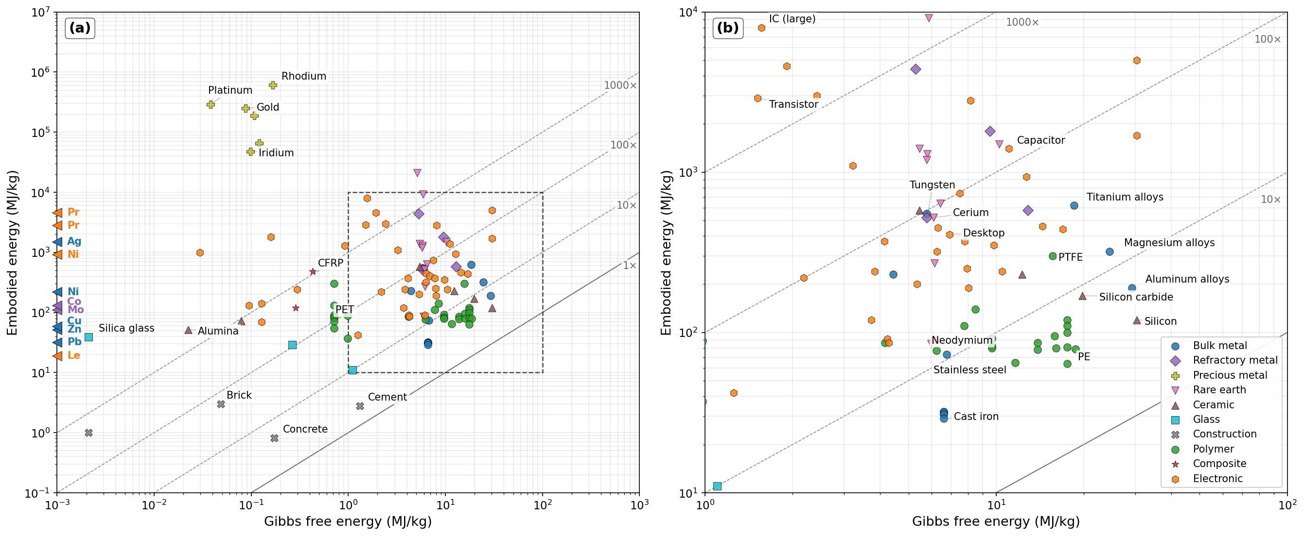
Most materials have Gibbs floors between a few MJ/kg and a few tens of MJ/kg, as determined by the basic thermochemistry of reducing elements from their naturally occurring forms. The exceptions are materials like cement, whose feedstock is already in the oxidation state of the finished product, and sulfide-derived metals like copper, where the oxidation of sulfur to sulfuric acid releases more energy than the metal reduction consumes, making the net Gibbs free energy negative.
Bulk industrial processes are already fairly close to their thermodynamic floors. The figure makes the gap look larger than it really is, because embodied energy is reported in primary-energy terms and includes the thermal-conversion inefficiencies of fossil-fueled electricity and heat. Under directly electrified inputs, much of that gap closes. World best practice energy intensity for iron and aluminum is within a factor of about two of the Gibbs floor (Worrell et al. (2008)), and these ratios have barely moved in decades of sustained engineering effort. Pushing energy efficiency closer to the thermodynamic floor typically requires more sophisticated equipment, such as additional heat-recovery stages, and more controlled reaction environments, which increases the physical capital cost of the plant itself. Improvement is often difficult even where current methods sit far above the floor; titanium, for example, is still made by the same energy-intensive process because every attempt to replace it has failed.
The gap between current embodied energy and the Gibbs floor varies widely by material. For some materials the gap is dominated by the thermodynamic cost of concentrating a dilute resource from bulk ore. As an example, mining copper requires processing roughly 200 tonnes of rock per tonne of metal, and the energy cost of that comminution dwarfs the synthesis chemistry (Ballantyne and Powell (2014)). For others, finite-rate process irreversibilities and heat losses account for most of the difference (Bejan (1996)), and further improvements are either difficult or uneconomical.
A minimal solar power system could pay back its embodied energy in days
Our aim is to estimate the embodied energy of a minimal energy production and transmission system, aggressively designed for rapid reproduction. Solar, fossil fuels, and nuclear could all in principle power a much larger economy; other options like wind or hydro are too limited in scale. At the physics floor, all three have payback times on a similar scale of days to weeks. We focus on solar because the other two have practical constraints that make them poor candidates for sustained rapid growth. Fossil fuels are finite in supply and produce CO\(_2\) emissions. Nuclear fission requires large individual facilities whose long construction times would impose substantial lags. Fusion would likely face even worse large-facility lags, and remains speculative.
A complete solar power system has three types of component, each with its own physical floor on embodied energy:
- Panel. The active absorber needs to be at least a few hundred nanometers thick to capture sunlight, but protecting this absorbing layer requires additional moisture barriers and polymer film.
- Electrical infrastructure. Collecting, converting, and transmitting power requires conducting material, and the mass required scales with the power carried and the distance.
- Storage. Storing energy for nighttime use requires a storage medium, and there is only a fixed amount of energy that can be stored per kilogram of material.
We design every component for one year of service rather than the twenty-five years typical of current solar installations. Today's silicon panels at utility scale take about a year to pay back their embodied energy, but most of their mass exists to support decades of outdoor durability. In an economy whose energy fleet doubles every few months, each cohort only needs to outlive its own replication time and so it is more efficient to create short-lived panels. Some components require technology that is not yet commercially scaled — most notably perovskite tandem absorbers — but the design is optimized to minimize energetic costs. The design was developed with the help of Claude Opus 4.7; Appendix I.1 works through each component in detail.
The table below shows the embodied energy breakdown and energy payback time for the complete system at different transmission distances, at both current embodied energies and the Gibbs floor.
| Current costs (MJ/W) | Gibbs floor costs (MJ/W) | Energy payback time (d) | |||||||||||
| Scenario | Panel | Elec. | Storage | Total | Panel | Elec. | Storage | Total | Current | Gibbs floor | |||
| No storage | |||||||||||||
| 0 km | 0.102 | 0.048 | — | 0.15 | 0.031 | 0.007 | — | 0.04 | 1.7 | 0.4 | |||
| 100 km | 0.103 | 0.130 | — | 0.23 | 0.031 | 0.037 | — | 0.07 | 2.7 | 0.8 | |||
| 500 km | 0.108 | 0.473 | — | 0.58 | 0.033 | 0.163 | — | 0.20 | 6.7 | 2.3 | |||
| 1000 km | 0.114 | 0.948 | — | 1.06 | 0.035 | 0.336 | — | 0.37 | 12.3 | 4.3 | |||
| 3000 km | 0.149 | 3.57 | — | 3.72 | 0.045 | 1.28 | — | 1.32 | 43.1 | 15.3 | |||
| With storage | |||||||||||||
| 0 km | 0.138 | 0.065 | 0.166 | 0.37 | 0.042 | 0.009 | 0.048 | 0.10 | 4.3 | 1.2 | |||
| 100 km | 0.139 | 0.111 | 0.167 | 0.42 | 0.042 | 0.027 | 0.048 | 0.12 | 4.8 | 1.4 | |||
| 500 km | 0.146 | 0.304 | 0.170 | 0.62 | 0.044 | 0.100 | 0.048 | 0.19 | 7.2 | 2.2 | |||
| 1000 km | 0.154 | 0.572 | 0.174 | 0.90 | 0.047 | 0.200 | 0.048 | 0.30 | 10.4 | 3.4 | |||
| 3000 km | 0.201 | 2.06 | 0.190 | 2.45 | 0.060 | 0.746 | 0.048 | 0.85 | 28.4 | 9.9 | |||
The energy payback time is sensitive to transmission distance: at 1000 km with storage, it is about 10 days at current embodied energies and 3 days at the Gibbs floor. Storage adds cost at short distances but saves conductor mass at long distances, with the crossover between 500 and 1000 km. While the precise numbers should not be taken too seriously, the embodied energies are spread across many materials and components and so an O(10-day) payback seems fairly robust even given the uncertainties. The Gibbs floor is roughly three to four times lower than current embodied energies across all configurations.
Energy payback is one constraint on a solar buildout. Material supply is another, and does not bind until the buildout is very large. The table below shows the mass of each potentially-constraining element required to build the system at four deployment scales, against world reserves and resources.
| Mass required for (Mt) | Global availability (Mt) | ||||||||
| Element | 18 TW (Current) |
100 TW | 1 PW | 6 PW (All land) |
Reserves | Resources | Dominant source | ||
| Carbon | 67 | 374 | 3,741 | 22,294 | 1,000,000 | \(\geq\)7,500,000 | coal, oil, gas | ||
| Cesium | 0.06 | 0.31 | 3.1 | 18.3 | \(\leq\)0.19 | — | pollucite | ||
| Copper | 15.9 | 88.4 | 884 | 5,269 | 980 | 1,500 | chalcopyrite porphyry | ||
| Iodine | 1.6 | 9.1 | 90.8 | 541 | 6.3 | \(\geq\)90,000 | caliche and brine deposits | ||
| Iron | 495 | 2,751 | 27,512 | 163,971 | 87,000 | \(\geq\)260,000 | hematite, magnetite, taconite | ||
| Lead | 1.1 | 6.1 | 60.6 | 361 | 95 | \(\geq\)2,000 | galena | ||
| Nickel | 4.7 | 25.9 | 259 | 1,546 | 140 | \(\geq\)350 | laterite, pentlandite sulfide | ||
| Tin | 0.22 | 1.2 | 12.4 | 73.9 | 6.0 | — | cassiterite | ||
| Zinc | 0.38 | 2.1 | 21.0 | 125 | 240 | 1,900 | sphalerite | ||
Reserves and resources are from USGS MCS 2026, while fossil carbon is from OPEC (2025) and the Energy Institute (2024). As we can see, iodine and cesium exhaust current reserves around 100 TW, a few doublings of world power. Iodine could be extracted from seawater if necessary, albeit at higher cost; obtaining cesium could be more challenging, but is only needed for the perovskite active layer; alternative designs with no cesium should be possible. Tin binds near 1 PW, while copper would begin to bind only once most land area has been covered and other elements are available in abundance.
As the payback time shrinks, supply-chain lags become the binding constraint
The EPBT calculation in the previous section divides cumulative energy out by cumulative energy in, with no attention to when the energy is committed. In reality, it takes time to process and transport materials, which means that this energy must be committed days or weeks prior to first power production. For an exponentially-growing economy, energy committed at lag \(\tau\) before delivery is more expensive by a factor of \(e^{\lambda \tau}\), and this decreases the maximum achievable growth rate.
To compute the lag-adjusted rate \(\lambda^*\), we estimate how far ahead of the system's first watt each step in the supply chain commits its energy, inflate that energy by \(e^{\lambda \tau}\), and solve the resulting fixed point. For now we assume the supply chain is co-located, so no material spends time in transit: the only lag is the time each material spends being physically transformed.
The table reports \(\lambda^*\) and the energy-weighted mean lag \(\bar\tau\) for each scenario; the per-step durations are in Appendix I.2 and the fixed-point calculation in Appendix H.2.
| Current | Gibbs floor | ||||||||
| Scenario | EPBT (d) | \(\bar\tau\) (d) | \(T_{\text{EPBT}}^{-1}\) (yr⁻¹) | \(\lambda^*\) (yr⁻¹) | EPBT (d) | \(\bar\tau\) (d) | \(T_{\text{EPBT}}^{-1}\) (yr⁻¹) | \(\lambda^*\) (yr⁻¹) | |
| No storage | |||||||||
| 0 km | 1.7 | 1.8 | 210 | 109 | 0.4 | 1.4 | 827 | 278 | |
| 1000 km | 12.3 | 2.1 | 30 | 26 | 4.3 | 2.2 | 85 | 59 | |
| With storage | |||||||||
| 0 km | 4.3 | 2.7 | 85 | 54 | 1.2 | 2.2 | 317 | 133 | |
| 1000 km | 10.4 | 2.4 | 35 | 29 | 3.4 | 2.4 | 107 | 68 | |
The mean lag is short because little time is required to physically manufacture and assemble the parts given an abundance of robotic labor, no transport delays, and just-in-time manufacturing. The longest individual steps are copper and nickel electrorefining at about a week each, but they feed mass-light components carrying little of the system's energy, so they barely move \(\bar\tau\). The diurnal cycle provides a hard floor, as a field commissioned at sunset cannot produce anything until sunrise.
Even with AGI, some dead time will occur at each link in the supply chain. We model it as a transport time, but it stands for every per-link delay not already counted in a step's processing — loading, storage, transfer, and literal transport alike. Figure 2 shows how the growth rate falls as we add a fixed such delay to every link in the supply chain, in our 1000 km scenario:
A few days per link would already outweigh the day or two of physical processing, so beyond short delays the lag is set by these per-link times rather than by fabrication. Even with ten days per link the shortest doubling time remains on the scale of weeks. With co-located factories and with AGI optimization I expect most delays could be reduced to less than a day, though some raw material might need to be transported longer distances.
Even counting the factories, energy production does not preclude doubling in weeks
So far we have estimated the energy required to expand the capacity of the electrical grid. But the grid is built by factories and machines that mine, smelt, manufacture, transport, and assemble everything, and building that capital takes energy too.
Consider a product that takes \(E_0 = 1\) MJ to make directly, on a machine that produces \(\mu = 1000\) units a day and took \(K = 10^5\) MJ to build. Spread over the output of a period \(t\), the machine adds \(K/(\mu t)\) to each unit, so the energy per unit is
\[
E = E_0 + \frac{K}{\mu t} = E_0 + \frac{E_1}{t}\,, \qquad E_1 = \frac{K}{\mu} = 100\ \text{MJ·day}.
\]
Most physical capital lasts many years or decades. If capital costs are amortized over this entire lifespan then \(t\gg 100\) days and thus capital contributions to the embodied energy are negligible, reducing costs to the \(E_0\) that we calculated in the previous section.
But in a rapidly growing economy we do not have time to amortize over the lifespan of the capital. If the economy grows exponentially at rate \(\lambda\), the average age of any piece of capital is \(\lambda^{-1}\) and thus the amortized cost becomes
\[
E = E_0 + \lambda E_1\,.
\]
For example, at a growth rate of 0.1 day⁻¹ the average age of any piece of capital is \(t = 10\) days and so we would find that \(E_1 /t = 10\) MJ, which is considerably greater than \(E_0\). The two contributions are equal at the breakeven time \(\tau = E_1/E_0 = 100\) days — the time a machine must run for the energy passing through it to equal the energy that built it, with
\[
E = E_0(1+\lambda \tau)\,.
\]
Amortized over longer than \(\tau\) the direct energy dominates, over shorter the capital does.
Building a solar grid takes many distinct processes, and each one is a machine of exactly this kind. Step \(i\) requires some direct energy, which on its own would add a time \(T_i\) to the payback time; it runs on capital with its own breakeven time \(\tau_i\), which inflates that contribution to \(T_i(1+\lambda\tau_i)\), just as the single machine's did. Summing over every step gives the total payback time:
\[
T_{\text{EPBT}} = \sum_i T_i\left(1+\lambda \tau_i\right) = T + \lambda S\,,
\]
where
\[
T = \sum_i T_i
\]
is the payback time if capital were free, and
\[
\qquad S = \sum_i T_i\tau_i
\]
accounts for the capital costs. The growth rate satisfies \(\lambda^{-1}\geq T_{\text{EPBT}}\), but \(T_{\text{EPBT}}\) itself rises with \(\lambda\), since faster growth leaves the capital younger and less amortized. Solving that self-consistently gives a quadratic in \(\lambda^{-1}\):
\[
\lambda^{-1} \geq \frac{ T +\sqrt{T^2+4S}}{2}\,.
\]
As described in Appendix I.3, we estimate breakeven times \(\tau_i\) for the various processes required to build the grid and then use this to compute \(S\) and \(\lambda\). For a 1000 km grid with storage, the ten largest contributions to \(S\) account for roughly 90% of the total and are as follows:
| Process | Direct \(T_i\) (d) | Breakeven \(\tau_i\) (d) | \(S_i = T_i\tau_i\) (d²) |
| Aluminum smelting cell | 2.97 | 16 | 46.1 |
| Transmission-tower fabrication | 0.37 | 78 | 28.9 |
| Silicon power-device fab | 0.12 | 151 | 17.3 |
| Copper smelt and refining | 0.38 | 21 | 7.9 |
| Fe-N-C catalyst pyrolysis | 0.05 | 150 | 7.5 |
| Final-leg transport fleet | 0.18 | 38 | 6.6 |
| Field-deployment fleet | 0.03 | 242 | 6.0 |
| Iron-air dry cooler | 0.19 | 28 | 5.2 |
| Iron-air cell assembly | 0.13 | 40 | 5.0 |
| Nickel refining | 0.41 | 12 | 4.9 |
| All other steps | 5.59 | — | 18.4 |
| Total | 10.4 | 15 | 154 |
From this, we can compute that \(\lambda \leq 20\) yr⁻¹, down from \(T^{-1} = 35\) yr⁻¹ if capital were free.
Extending to all four designs, with the no-storage cases carrying a peak-sizing penalty on their daylight-only building capital:
| Growth bound (yr⁻¹) | Doubling bound (d) | ||||||
| Scenario | \(T\) (d) | \(S\) (d²) | No lag | Lagged | No lag | Lagged | |
| 0 km, no storage | 1.7 | 77 | 38 | 27 | 6.7 | 9.2 | |
| 0 km, with storage | 4.3 | 66 | 35 | 25 | 7.3 | 10 | |
| 1000 km, no storage | 12.3 | 443 | 13 | 11 | 19 | 23 | |
| 1000 km, with storage | 10.4 | 154 | 20 | 16 | 13 | 16 | |
The lagged columns also charge the time it takes to build the factories, on top of the supply-chain lags carried over from the previous section. A plant has to produce its own materials, be assembled, and be brought up to operating temperature before it makes anything, and that delay inflates its embodied energy by the same \(e^{\lambda\tau}\) those lags carry. We estimate each plant's build time from its bill of materials, as worked through in Appendix I.3.
The estimates so far assume co-located production. In practice the materials feeding both the grid and the factories that build it move between processing steps, and every leg adds dead time. Figure 3 shows the bound falling with transport and dead time per link for all four designs, charging transport on the grid's materials and the factories' alike. Across all four designs the shortest doubling time stays between about ten days and a month, even allowing twelve days of transport delay on every link in the chain.
Discussion
A minimal solar generation and distribution system, designed for fast reproduction rather than long service, can generate enough energy to reproduce itself on the scale of weeks. That holds even after including construction lags, the transport of materials, and the physical capital of the factories that build it. That is an order of magnitude faster than present-day energy production. The system is not especially sophisticated. It needs abundant robot labor and a few technologies that are not yet deployed at scale, most notably perovskite tandem cells, but the main lever is just optimizing for low material use and accepting short lifetimes in return.
Whether the whole economy can double this fast turns on whether some other sector binds harder than energy. Given our estimated costs for mining and smelting in the appendices, and payback times for the associated sectors in present-day input-output tables, I think these are unlikely to substantially slow growth. However, creating more complex machinery like transportation devices, robots, and silicon chips requires much longer supply chains and more advanced manufacturing processes. It seems plausible that these could be more constraining, but they are harder to reason about from first principles than energy production or bulk resource acquisition.
Could it go faster still? Biology shows that much faster self-replication is possible. The fastest cyanobacteria and microalgae double every couple of hours in good conditions. But they cannot generate electricity, hold stable macroscopic structure, or move energy over long distances, so nothing algae-like could power a real economy.
Advanced nanotechnology need not share biology's limitations, but it does not escape the physics either. A nanotech system that stores power overnight and moves it across the country pays the same storage and transmission costs that dominate our estimate; its batteries are bound by the same bond energies and its conductors by the same transport physics, and it stays in the weeks-scale regime we have estimated. But if the nanotechnological economy can avoid transport and perform all of its tasks locally, then the binding constraint becomes the thickness of the solar panels themselves, and we cannot rule out doubling times of several days for energy production from energetic cost considerations alone.
Appendix H: Mathematical foundations
H.1 Payback time and the growth bound
In Part 1, Appendix A, we introduced the input-output description of the economy, in which the matrices \(A\), \(B\), and \(\Delta\) record, per unit of a sector's output, the intermediate inputs it consumes, the capital it holds, and the capital that wears out each year. With all output reinvested, the maximum growth rate \(\lambda\) satisfies the eigenvalue equation:
\[
(I - A - \Delta)\,y = \lambda B y,
\]
where the associated eigenvector \(y\) gives the distribution of sectors that maximizes growth. We can rearrange it into the more conventional eigenvalue form
\[
y = \lambda M y\,,
\]
where we introduce the matrix
\[
\begin{aligned}
M &= (I-A-\Delta)^{-1}B \\
&= \left[I + (A+\Delta)+(A+\Delta)^2+\dots\right]B\,.
\end{aligned}
\]
Examining this series, we see that the matrix entry \(M_{ij}\) is the total output of sector \(i\) required to build and maintain the capital behind one unit of sector \(j\)'s output. In particular, the diagonal entry \(M_{ii}\) gives the total output of sector \(i\) required to increase that sector's production rate by a unit amount, which is simply the payback time for the sector.
Every entry of \(M\) is non-negative, so by the Perron-Frobenius theorem it has a unique largest eigenvalue \(\rho(M)=\lambda^{-1}\) with a strictly positive eigenvector. For any other matrix \(N\) that satisfies
\[
M_{ij}\geq N_{ij}\geq 0
\]
for every entry, it is straightforward to show that
\[
\rho(M)\geq\rho(N)\geq0\,.
\]
If we only estimate some entries of \(M\) and set the remainder to zero, the resultant matrix \(\tilde M\) will thus provide us with an upper bound on the growth rate:
\[
\lambda = \rho(M)^{-1}\leq\rho(\tilde M)^{-1}\,,
\]
and, in particular,
\[
\lambda \leq \frac 1 {M_{ii}}
\]
for every sector in the economy.
In the main text, we focus on the energy production sector \(e\), with the energy payback time corresponding to \(M_{ee}\). This payback time includes all of the energy required to manufacture and assemble the various components of the power grid, given the requisite machinery and other physical capital, but does not include the costs of that capital. Those costs are included in the off-diagonal entries \(M_{ei}\), which gives the energy required to increase sector \(i\)'s output, and the column entry \(M_{ie}\) which tells us how much of sector \(i\) output is needed to increase energy production. Setting all other entries of \(M\) to zero, we thus find that:
\[
\lambda^{-1}\geq\frac{M_{ee} + \sqrt{M_{ee}^2 + 4\sum_{i\neq e} M_{ei}M_{ie}}}{2}\,,
\]
which, with \(T = M_{ee}\) and \(S = \sum_{i\neq e}M_{ei}M_{ie}\), is equivalent to the quadratic growth bound used in the main text.
H.2 Inputs committed at distributed times
The most general way to treat lags is to let the input-output coefficients depend on the time \(\tau\) between an input being committed and the output it serves appearing. In place of the constant matrices of H.1 we have kernels \(A(\tau)\), \(\Delta(\tau)\), and \(B(\tau)\), and the material balance becomes
\[
y(t)\geq \int d\tau \,\left[A(\tau)y(t+\tau)+\Delta(\tau)y(t+\tau)+B(\tau)\dot y(t+\tau)\right]\,,
\]
with each flow referenced at the time \(t+\tau\) of the output it serves rather than the earlier time it is committed. For the maximal-growth solution \(y(t) = y e^{\lambda t}\), every shifted flow becomes \(y(t+\tau) = e^{\lambda\tau}y(t)\), and we find that
\[
[I-\hat A(\lambda)-\hat\Delta(\lambda)]y = \lambda \hat B(\lambda) y\,,
\]
where we define
\[
\hat A(\lambda) = \int d\tau\,e^{\lambda\tau}A(\tau)\,,\qquad \hat \Delta(\lambda) = \int d\tau\,e^{\lambda\tau}\Delta(\tau)\,,\qquad \hat B(\lambda) = \int d\tau\, e^{\lambda\tau}B(\tau)\,.
\]
We can collect these lagged operators into a matrix
\[
\hat M(\lambda) = [I - \hat A(\lambda) - \hat\Delta(\lambda)]^{-1}\hat B(\lambda)
\]
so that the maximum growth rate satisfies:
\[
y =
\lambda \hat M(\lambda)y\,.
\]
As in the previous section, we can upper bound \(\lambda\) by considering the diagonal payback times:
\[
\lambda^{-1}\geq \hat M_{ee}(\lambda)\,.
\]
Rearranging the infinite series that defines \(\hat M(\lambda)\), it is straightforward to show that
\[
\hat M_{ee}(\lambda) = T_{\text{EPBT}}\int f(\tau)e^{\lambda \tau}\,d\tau
\]
where \(T_{\text{EPBT}}\) is the lag-free energy payback and \(f(\tau)\) gives the fraction of this energy that must be committed at lead time \(\tau\). We thus find that
\[
1 \geq \lambda\,T_{\text{EPBT}}\int f(\tau)\,e^{\lambda\tau}\,d\tau\,,
\]
which we can solve numerically to bound \(\lambda\).
Appendix I: The solar electricity system
I.1 System design
The main text described the system as three components — the panel, the electrical infrastructure, and storage. This appendix sizes each in detail, designing every component to the minimum mass that still does its job for a year. The electrical infrastructure splits into three stages along the path the power takes. Collection cabling gathers the current from the panels, a converter steps the voltage up, and a trunk line carries it to where it is used. A closing section covers transporting and installing the materials.
I.1.1 Panel
The aim is to make every layer of the panel as thin as physics allows. Per-kilogram embodied energy sits within an order of magnitude across condensed-matter materials, while layer thicknesses vary by orders of magnitude. Mass per square meter is therefore the dominant lever for embodied energy, and the minimum-embodied-energy design pushes each layer to its functional floor.
The result is a thin polymer film, more like agricultural plastic mulch than a conventional solar module. It rolls out across the ground and is anchored with steel U-staples. Inside the polymer sandwich the active layers form a tandem cell, two perovskite absorbers stacked so the top captures visible light and the bottom the near-infrared that passes through. Thin aluminum oxide moisture barriers and silica abrasion-resistant hardcoats protect each face.
The table below gives the full bill of materials, top-to-bottom from the sun-facing side. Layers that appear twice in the stack — on both faces of the panel, or in both junctions of the tandem cell — are marked (×2), with mass and thickness shown as totals across both instances. The columns headed ε give each layer's embodied energy per kilogram: ε current for what today's processes spend to produce and form it, and ε Gibbs for the thermodynamic floor introduced in the materials section above. These figures include fabrication costs, such as extruding and laminating the polymer films or depositing the thin active layers, though typically such costs are small compared to costs for the chemical processes. The columns headed E give mass × ε, the energy that layer contributes per square meter of panel, shown both at current processes and at the floor.
| ε (MJ/kg) | E (MJ/m²) | |||||||
| Layer | Thickness | Mass (g/m²) | current | Gibbs | current | Gibbs | Purpose | |
| Silica hardcoat (×2) | 2.0 μm | 4.0 | 15 | 0.002 | 0.060 | 0 | scratch / abrasion resistance | |
| Aluminum oxide barrier (×2) | 2.0 μm | 6.0 | 200 | 0.02 | 1.20 | 0 | moisture barrier | |
| Polypropylene front sheet | 12 μm | 10.8 | 28 | 16 | 0.30 | 0.17 | mechanical + UV protection | |
| Polyolefin elastomer encapsulant | 50 μm | 43.2 | 28 | 17.5 | 1.21 | 0.76 | binds cell layers, impact buffer | |
| AZO transparent top contact | 100 nm | 0.71 | 100 | <0 | 0.071 | 0 | top electrode | |
| Tin oxide electron transport (×2) | 60 nm | 0.42 | 30 | 0.09 | 0.013 | 0 | electron extraction | |
| Wide-bandgap perovskite absorber | 0.5 μm | 2.14 | 60 | <0 | 0.13 | 0 | upper junction (visible) | |
| Copper recombination contact | — | 0.05 | 37 | <0 | 0.002 | 0 | current matching between junctions | |
| Narrow-bandgap perovskite absorber | 0.5 μm | 2.65 | 60 | <0 | 0.16 | 0 | lower junction (NIR) | |
| Nickel oxide hole transport (×2) | 50 nm | 0.24 | 45 | 2 | 0.011 | 0 | hole extraction | |
| Carbon back contact | 3.0 μm | 4.5 | 15 | 0 | 0.068 | 0 | back electrode | |
| Polyethylene back sheet | 15 μm | 13.8 | 28 | 17.5 | 0.39 | 0.24 | mechanical, weather seal | |
| Steel staples | — | 11 | 13 | 7 | 0.14 | 0.077 | wind-load anchoring | |
| Film extrusion + lamination | — | — | — | — | 0.32 | 0 | ||
| Total | 99.5 | 4.08 | 1.24 | |||||
Entries marked "<0" are materials whose Gibbs free energy of synthesis from natural feedstock is technically negative: sulfide ores release more energy on oxidation to sulfuric acid than the metal reduction absorbs, and perovskite synthesis from elemental Pb, I, and Cs is slightly exothermic. In practice these floors are not approached because ore extraction and finite-rate process losses dominate.
Most of the panel's embodied energy is in the polyolefin and polypropylene polymer sheets — the front sheet, the encapsulant, and the back sheet — which together account for about half the total. These layers give the panel mechanical strength against thermal cycling and handling stress, and shield the active layers from UV degradation. The next-largest contributor is the aluminum oxide moisture barrier on each face, which keeps water away from the perovskite over a year of outdoor service. The per-kilogram energies for the deposited layers include the deposition step itself: each is built up from its Gibbs floor with a mature-process multiplier, and the barrier is costed for sputtering or atmospheric-pressure CVD rather than the slower atomic layer deposition used in flexible electronics today.
The perovskite absorbers themselves are only a small contributor to the panel's embodied energy. At 0.5 μm each, they barely register in mass terms, and they are not particularly energy intensive to make per unit mass. Their thickness is set by optical absorption: perovskite's band-edge absorption coefficient near \(10^5\) cm⁻¹ means 0.5 μm absorbs about 99% of above-bandgap photons in a single pass, with comfortable margin against fabrication non-uniformity.
The module could operate at perhaps 25% efficiency under standard test conditions. Record perovskite/perovskite tandem cells have reached 28% in the lab (NREL Best Research-Cell Efficiency Chart); after cell-to-module losses, module efficiency comes in at 22–25%, against a Shockley-Queisser ceiling of about 46% for an ideal two-junction tandem (De Vos (1980)).
At a well-insolated site, average incident sunlight over the 24-hour cycle is about 200 W/m². With a 0.8 performance ratio — accounting for dust soiling, operating temperature above the 25 °C of standard test conditions, spectral mismatch, and resistive losses in module-internal wiring — the panel delivers \(200 \times 0.25 \times 0.8 \approx 40\) W/m² of average delivered power. Losses in the collection cable, the power converter, and the trunk transmission line are accounted for separately in the sections that follow.
I.1.2 Collection cabling
Each sub-field is about one hectare, with a converter at its center. An insulated copper cable carries the panels' current the 30–50 m to it, sized by the current it must carry, thick enough that the peak noon current does not overheat it. Running the panels at 1500 V, the standard maximum for DC solar, keeps that current low and the cable thin. The mass breakdown, per m² of panel:
| ε (MJ/kg) | E (MJ/m²) | ||||||
| Component | Mass (g/m²) | current | Gibbs | current | Gibbs | Purpose | |
| Copper edge busbars | 0.1 | 37 | <0 | 0.004 | 0 | extracts current at panel edge | |
| Copper collection cable | 10 | 37 | <0 | 0.37 | 0 | carries current to converter | |
| XLPE insulation | 3 | 29 | 17.5 | 0.088 | 0.053 | 1500 V voltage isolation | |
| Forming | — | — | — | 0.05 | 0 | wire drawing and insulation extrusion | |
| Total | 13 | 0.51 | 0.053 | ||||
The copper cable dominates. Its insulation is thin, about 0.9 mm of cross-linked polyethylene to hold the 1500 V. Collection comes to about 12% of the panel's embodied energy. The cable is sized for the peak current, not the average, so adding storage and oversizing the panel field to charge it scales the collection mass up in step.
I.1.3 Power conversion
A solar field collects its power at 1500 V, but moving that power any distance needs a much higher voltage to keep the transmission conductor thin (I.1.4). A power converter bridges the two, stepping the voltage up. Each sub-field has a solid-state converter at its center. Its mass breakdown, per m² of panel:
| ε (MJ/kg) | E (MJ/m²) | ||||||
| Component | Mass (g/m²) | current | Gibbs | current | Gibbs | Purpose | |
| Copper windings | 13.5 | 37 | <0 | 0.50 | 0 | carries primary and secondary current | |
| Amorphous-iron core | 5.4 | 45 | 6.6 | 0.24 | 0.036 | magnetic flux path between windings | |
| Aluminum heat exchanger | 4.9 | 76 | 29 | 0.37 | 0.14 | removes switching and core losses | |
| Silicon switching devices | 4.0 | 66 | 8.0 | 0.26 | 0.032 | chops input current at 2 kHz | |
| Carbon-steel enclosure | 2.6 | 13 | 6.6 | 0.034 | 0.017 | structural housing and EMI containment | |
| Winding and assembly | — | — | — | 0.02 | 0 | ||
| Total | 30.4 | 1.43 | 0.23 | ||||
The copper windings are the largest single cost. Their cross-section is set by the current they carry. At 7 A/mm² with liquid cooling, the wire holds a safe temperature over a year of service.
A converter today would use silicon carbide switches, but device-grade silicon carbide grows too slowly to reproduce in a fast-doubling economy, so we use silicon and accept a core about 2.7 times heavier. The converter comes to about a third of the panel's embodied energy, at a power density consistent with demonstrated solid-state transformers (Huber and Kolar (2019), Leibl, Ortiz and Kolar (2017)).
Like the collection cabling, the converter is sized for peak power rather than average. The silicon switches must handle the noon current, and storage downstream does not relax that.
I.1.4 Transmission
A transmission line requires a conductor to carry the current and insulation to prevent discharge to its surroundings. For a DC line carrying power \(P\) over distance \(D\), the fractional resistive loss is
\[
f_L = \frac{P \rho D}{2 V^2 A},
\]
where \(\rho\) is the resistivity of the conductor, \(A\) its cross-section, and \(V\) the per-pole voltage — 500 kV for the ±500 kV bipole used below. The conductor cross-section needed at a given loss target therefore scales as \(1/V^2\).
The ideal conductor maximizes conductance per unit of embodied energy. We use aluminum, the standard choice in essentially all transmission lines today; it self-passivates and hangs bare from the towers, with no insulating jacket. Sodium is somewhat better by that measure and was deployed in jacketed distribution cables in the 1960s, but its low melting point and water reactivity make it somewhat less practical, and the saving is modest.
There are two ways to insulate against the operating voltage: hold the conductor far enough from the ground that the air gap does not break down (overhead, on towers), or wrap it in a solid insulator (polymer jacket, laid on the ground). Either way, insulation cost grows with voltage — taller towers are heavier, thicker polymer is heavier — while conductor cost falls as \(1/V^2\). The total has a minimum at an intermediate voltage, around ±500 kV for overhead; the minimum is shallow, and choices within its flat region move the total by tens of percent. At the overhead optimum, per kW·km of power carried:
| ε (MJ/kg) | E (MJ/kW·km) | ||||||
| Component | Mass (g/kW·km) | current | Gibbs | current | Gibbs | Purpose | |
| Aluminum conductor | 2.9 | 76 | 29 | 0.218 | 0.084 | carries current at ±500 kV | |
| Steel messenger wire | 0.2 | 13 | 6.6 | 0.003 | 0.001 | mechanical support of conductor | |
| Steel lattice towers | 13.0 | 13 | 6.6 | 0.169 | 0.086 | holds line at operating height | |
| Porcelain insulators | 0.08 | 11 | 0.02 | 0.0009 | 0.000 | hangs conductor from towers | |
| Forming | — | — | — | 0.049 | 0.000 | aluminum extrusion and stranding + tower fabrication (Ashby B6) | |
| Total | 16 | 0.44 | 0.16 | ||||
The cross-section set by the formula above assumes a steady current. But a no-storage line carries the panels' raw output, zero at night and peaking at noon, and resistive loss grows with the square of the current, so holding the same loss target costs extra conductor. For a half-sine daily profile the penalty is \(\langle I^2 \rangle/\langle I \rangle^2 = \pi^2/4 \approx 2.5\), and a no-storage trunk needs about 2.5 times the conductor of a steady line carrying the same average power.
I.1.5 Storage
The total energy that can be stored in matter is limited by the strength of the chemical bonds holding the matter together. If you exceed this, the material will break. These same bond energies also determine the cost of producing the material in the first place. As a result, the embodied energy per stored energy capacity for a device tends to be much larger than one. The only way around this is to use a storage medium that is essentially free.
We use iron-air batteries. These reduce hematite — the most abundant iron ore on Earth — to metallic iron by alkaline electrolysis on charge, and re-oxidize the iron to Fe(OH)₂ in air on discharge. Hematite is essentially free, so the iron half of the cell is cheap. A minimal design for one-year service with daily cycling could look something like the following per MJ of storage delivered:
| ε (MJ/kg) | E (MJ/MJ) | ||||||
| Component | Mass (g/MJ) | current | Gibbs | current | Gibbs | Purpose | |
| Iron ore concentrate (Fe₂O₃) | 480 | 0.15 | 0.01 | 0.073 | 0.005 | active material | |
| First-charge formation energy | — | — | — | 1.44 | 0.64 | unrecovered Fe³⁺ → Fe⁰ at commissioning | |
| KOH electrolyte | 65 | 3.7 | 0.81 | 0.24 | 0.053 | ionic conduction | |
| Carbon black gas-diffusion layer | 22 | 8 | 0 | 0.18 | 0 | air-electrode substrate | |
| Fe-N-C ORR catalyst | 2 | 50 | 0 | 0.10 | 0 | O₂ reduction catalyst | |
| Sintered Ni mesh + NiFeOOH OER | 6 | 135 | <0 | 0.81 | 0 | O₂ evolution catalyst | |
| Steel collectors / bipolar plates | 9 | 13 | 6.6 | 0.12 | 0.060 | current collection | |
| FeS₂ hydrogen-evolution suppressant | 4 | 3 | 3.1 | 0.012 | 0.012 | suppresses H₂ evolution | |
| Na₂S corrosion-suppressant additive | 2 | 12 | 5.4 | 0.024 | 0.011 | suppresses corrosion | |
| Polyethylene housing and gaskets | 7 | 28 | 17.5 | 0.20 | 0.12 | containment and seal | |
| Carbon-steel dry-cooler thermal management | 31 | 12 | 6.6 | 0.37 | 0.20 | rejects ~280 kW cycle-avg heat per sub-field | |
| Assembly | — | — | — | 0.25 | 0.013 | construction energy | |
| Total | 628 | 3.8 | 1.1 | ||||
The first-charge formation energy is the largest single cost. In normal operation, the cell cycles iron between Fe(OH)₂ and metallic Fe, transferring two electrons per atom. But the iron is loaded as hematite (Fe₂O₃), with the iron at a higher oxidation state still. Reducing it to metallic iron at commissioning takes three electrons per atom, and the extra one is paid once and never recovered.
The cell charges at about 1.55 V and discharges at about 1.0 V. That voltage gap, set by overpotentials at the two oxygen electrodes, gives a voltaic efficiency of about 65%, and coulombic and parasitic losses pull the round-trip down to about 55%. Sealed chemistries like lead-acid or lithium-ion avoid this and run at 85–90% but embody an order of magnitude more material per MJ stored. The biggest open assumption is Fe-N-C catalyst durability over the one-year service window. The catalyst has only been demonstrated over hundreds of hours, and falling back to simpler catalysts brings the efficiency to about 50%.
While alternative options for cheap power storage exist, they suffer other limitations. Pumped hydro and compressed-air storage at suitable geology can come in below 1 MJ per MJ, but viable reservoirs and salt caverns are scale-limited well short of what a self-replicating economy needs. Thermal storage in bulk rock or sand isn't site-limited, but the heat exchangers and turbines needed to convert it back to electricity bring the cost back to above 1 MJ per MJ, and the round-trip efficiency is low.
I.1.6 Transport and field deployment
Appendix B of Ashby (2021) gives the following estimates of the energetic cost to transport freight:
| Mode | Energy (MJ/t·km) |
| Container ship (very large) | 0.04 |
| Bulk carrier | 0.11 |
| Rail freight (electric) | 0.22 |
| 40-tonne truck | 0.82 |
| Long-haul aircraft | 6.5 |
We take 0.3 MJ/t·km as an order-of-magnitude estimate of transportation costs, comparable to current rail costs. Slower transportation requires less energy but also increases time lags and physical capital requirements. The distances that the intermediate and final products must move depend on the specific geographical setup; for simplicity we assume an average of 1000 km which then increases the embodied energy of every component by 0.3 MJ/kg, generally negligible compared to production.
Once transported, the components must be installed. We cost the deploying machines as a roughly 1 kW field robot working for the time a human crew would take — the per-tonne install hours are from the man-hour tables in Storm (2019), so the deployment energy is just those hours run at 1 kW — with the panel laid continuously by its own rig instead:
| Component | Install (h/t) | Field deployment (MJ/kg) |
| Solar panel | rig | 0.043 |
| Collection cable | 5 | 0.018 |
| Power converter | 10 | 0.036 |
| HVDC trunk cable | 6 | 0.022 |
| Transmission tower | 24 | 0.086 |
| Insulator string | 30 | 0.108 |
| Iron-air cell | 8 | 0.029 |
Again these costs are negligible compared to those required for producing the materials.
I.2 Lag inventory
The energy a step consumes is spent before the system makes any power, and it has to wait out not just that step but every step downstream of it. A step's lead time is therefore its own duration plus the durations of everything downstream. Collected into the energy-weighted lag distribution \(f(\tau)\), these give the maximum-rate bound from Appendix H.2,
\[
1 = \lambda\,T_{\text{EPBT}}\int f(\tau)\,e^{\lambda\tau}\,d\tau.
\]
With robotic labor, just-in-time scheduling, and a co-located chain, a step's duration is just the time the material spends being transformed. Most steps are throughput-limited and take a few hours; the ones that take longer are rate-limited by chemistry, heat, or the day-night cycle:
| Step | Duration (d) | What sets it |
| Copper / nickel electrorefining | 7 | deposition current density, held low to suppress dendrites |
| Storage deployment | 2 | field install, first charge, and wait for sunrise |
| Overhead-line deployment | 1.5 | span erection and commissioning |
| Panel-field deployment | 1 | layout and wait for sunrise |
| Porcelain firing | 1 | kiln firing and cooldown |
| Aluminum electrolysis | 1 | molten cryolite bath turnover |
| Billet cooling | 0.75 | air-cooling cast steel to a handleable temperature |
| Polymer cracking | 0.5 | reaction residence |
About two-thirds of the committed energy sits at the one-to-two-day deployment floor, set by the wait for sunrise. Copper and nickel electrorefining, though the longest steps, feed thin conductors and contacts carrying about 4% of the energy, so they add only a small high-lag tail.
I.3 Physical capital requirements
The breakeven time of a plant is the energy \(K_i\) embodied in it divided by the rate \(f_i\) at which energy flows through it,
\[
\tau_i = \frac{K_i}{f_i}\,.
\]
To estimate \(K_i\) we use Claude Opus 4.8 to size the lightest plant that performs the step at today's process efficiency and lasts one year. One year comfortably exceeds the reproduction time, so the design is conservative; a faster-doubling fleet would replace each plant before it wore out and could build it lighter still (though in practice I think gains from pushing to even shorter lifespans are limited).
As an example, take the aluminum cell that makes the conductor metal. A Hall-Héroult pot built to last a year is a steel shell on a concrete pad, holding a molten cryolite bath with carbon electrodes and fed by its own rectifier; a plausible bill of materials is:
| Component | Material | Mass (kg) | ε (MJ/kg) | Energy (GJ) |
| Carbon anode and cathode blocks | Graphite | 44,850 | 35 | 1,570 |
| Pot shell, cradle, collector bars, hoods | Carbon steel | 27,000 | 13 | 360 |
| DC busbar and rectifier aluminum | Aluminum | 4,290 | 76 | 327 |
| Molten cryolite working inventory | Na₃AlF₆–AlF₃ | 14,000 | 15 | 210 |
| Furnace lining | Firebrick | 24,700 | 3 | 74 |
| Foundation pad | Concrete | 86,400 | 0.8 | 71 |
| Rectifier windings, switches, core | Cu / Si / Fe | 540 | — | 22 |
| Total \(K\) | 2,630 |
The pot turns out about 810 t of aluminum a year, which carries roughly 62 TJ of embodied energy, while the pot itself embodies 2.6 TJ. It therefore breaks even after \(\tau = 2.6\,\text{TJ} / 62\,\text{TJ·yr}^{-1} \approx 15.5\) days. By creating similar breakdowns for all 36 processes needed to produce the solar grid, we can produce the estimates of \(\tau_i\) and \(S\) found in the main text.
The breakeven times we estimate are design targets, and it is worth comparing them against the same quantity in today's economy. For a sector of the 2017 input-output tables, the analog of \(\tau_i\) is the embodied electricity in the sector's capital stock divided by the embodied electricity in its annual intermediate flow, computed on the same electrified, emergency-utilization configuration as the main text. The table compares the ten largest contributors against their sector analogs:
| Process | Breakeven \(\tau_i\) (d) | BEA sector analog | Sector breakeven (d) | Ratio |
| Aluminum smelting cell | 16 | Alumina and primary aluminum | 38 | 2.4 |
| Transmission-tower fabrication | 78 | Coating and heat treating | 84 | 1.1 |
| Silicon power-device fab | 151 | Semiconductors | 235 | 1.6 |
| Copper smelt and refining | 21 | Nonferrous smelting and refining | 72 | 3.4 |
| Fe-N-C catalyst pyrolysis | 150 | Other basic inorganic chemicals | 103 | 0.7 |
| Final-leg transport fleet | 38 | Truck transportation | 732 | 19 |
| Field-deployment fleet | 242 | Nonresidential maintenance | 68 | 0.3 |
| Iron-air dry cooler | 28 | Air-conditioning and heating equipment | 88 | 3.1 |
| Iron-air cell assembly | 40 | Storage battery manufacturing | 42 | 1.0 |
| Nickel refining | 12 | Nonferrous smelting and refining | 72 | 6 |
Most of the plants are assumed only modestly lighter than their present-day sector analogs, between one and six times, and two are heavier. The one large gap is transport, where the sector figure reflects today's duty cycles and the designed fleet runs around the clock. The field-deployment fleet comes out heavier than its analog because today's construction does with labor what the design must do with capital. The comparison is rough: a BEA sector is a dollar-weighted basket of many processes, so a single plant inherits its parent sector's average recipe, and the utilization adjustment does not reach non-manufacturing sectors like trucking.
We can also run the whole calculation at today's capital intensities. Substituting the system's bill of materials, valued at 2017 producer prices, into the input-output tables, so that the factories and their upstream supply chains carry the capital of today's economy wholesale, gives a bound of 7.8 yr⁻¹ for the 1000 km storage design, a doubling time of 32 days against the 13 days of the main text. Part of the difference is the lighter plants; part is that the input-output substitution also charges upstream sectors that the minimal chain does not require. Even built with today's factories, the system could double in about a month.
The breakeven times above carry no lags. But like every other input, a plant's embodied energy must be committed before the plant is operational, and energy committed a time \(t\) ahead is more expensive by a factor \(e^{\lambda t}\). The same correction applies to the factories as to the grid they build. With 36 distinct plants, though, tracing each one's supply chain in the same detail is impractical, so we simplify. For each plant we estimate the total time to build it and assume its energy is committed evenly across that time, which inflates its contribution by the average of \(e^{\lambda t}\) over the build.
We had Claude estimate the build time for each plant, split into three parts: producing the plant's own materials, constructing and assembling the facility, and commissioning it. Producing the materials takes a day or two and the construction and assembly a week or two; commissioning is quick except for the high-temperature plants, which must bring their refractory lining up to temperature slowly enough not to crack it, adding one to two weeks. In all the build runs two to three weeks for most plants, and up to five for the hottest, the aluminum cell and the porcelain kiln.