
The AI Industrial Explosion — Part 6: Choke points to growth?
In Part 2, we examined how quickly the US could transition to rapid growth after AGI, starting from today’s economy, and found that energy production could double in about five years. People often have the intuition that a few narrow choke points, such as chips, robot parts and the rare-earth minerals they use, or power production, would delay this, because the economy would have to wait while their supply is built up. Part 2 couldn’t test this, since it divided the economy into only 71 sectors, too coarse to see these supply chains. Here, we use a finer decomposition of the economy and of these supply chains to show that none of these choke points actually matter that much.
Throughout, we work in the same framework as Part 2. We assume AGI arrives at year zero, and that from then on we know the algorithms to run AI workers and how to build the robots they need. The economy is still bottlenecked on actually producing things. Every new chip and robot, and every factory that makes them, has to be made by industries that start at today’s US capacity and take time to expand. We count only the time to physically build and ramp up each plant, leaving out permitting, siting, and order queues.
We also assume the economy grows as fast as it can, holding consumption at today’s level and reinvesting everything else. This is unrealistic, but since we’re analyzing whether choke points matter rather than forecasting prices, I think it is mostly benign. Consumption slows growth, which makes choke points less important, because there’s simply more time to build things with long lead times.
We begin by showing that the economy grows basically as fast with the 401-sector decomposition as with the 71-sector one, and look at prices. Shortages move prices far more than output, but prices are very sensitive to assumptions and cannot be reliably forecast. We then discuss, in turn, the chip supply chain, robotics, and power production.
Shortages move prices far more than output
In Part 2 we used BEA’s 71-sector summary tables. By improving our solving methods, we have been able to upgrade to the 401-sector detailed tables. To a first approximation, it doesn’t matter. Figure 1 repeats Part 2’s sector trajectories at both resolutions, at emergency utilization with a half-year construction lag. The 401-sector economy is somewhat slower, by a few tenths of a year, and then grows at the same rate.
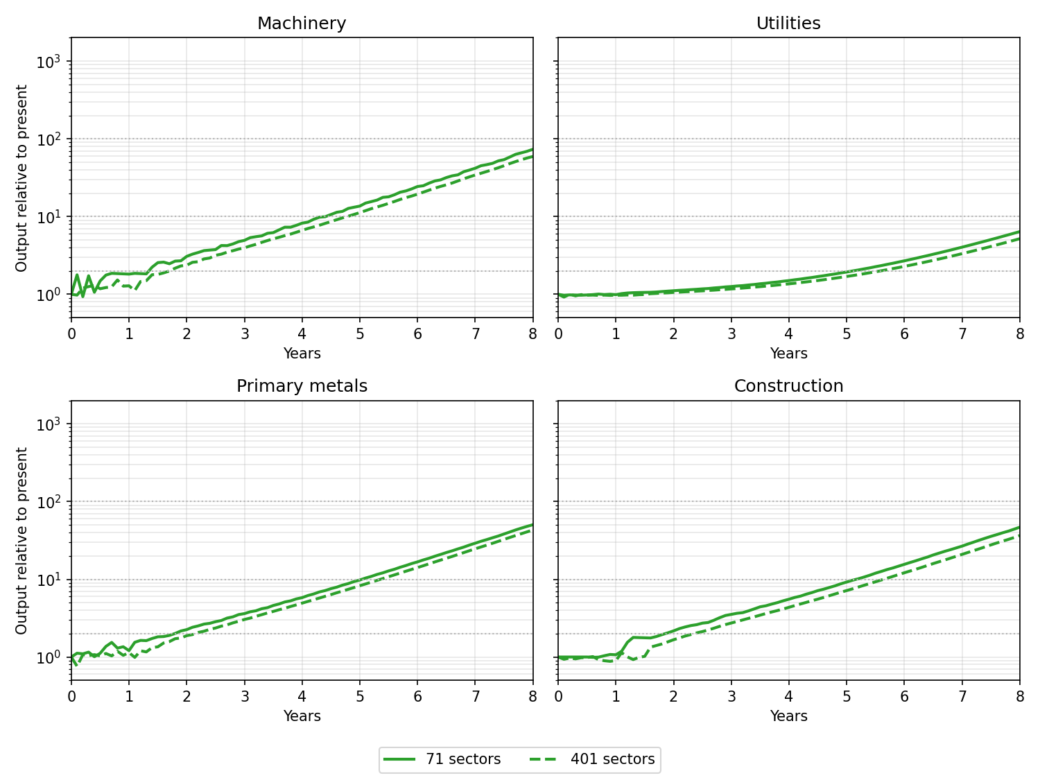
Figure 1. Output relative to present for four key sectors in the 71-sector and 401-sector models (emergency utilization, half-year lag).
In the series so far, we have focused on quantity of production rather than on prices. Prices depend on scarcity, which makes them much more sensitive to assumptions. Imagine slightly more left gloves than right gloves. A right glove is then worth a whole pair, and a left glove nothing. Add a few right gloves and the prices swap, though hardly any more pairs are made. Likewise, in the economy goods in short supply become expensive while goods in surplus become cheap. Construction and research lags, patents and regulatory barriers, investor behavior, plain chance, and much else outside our model can change which goods are short, and so move prices a lot while barely changing what is actually produced.
Nevertheless, our model does allow us to compute prices, or so-called shadow prices, that in an idealized world would reflect the true prices of goods. We explain how to compute them in Appendix J.
Figure 2 shows the shadow prices of some key goods over time:
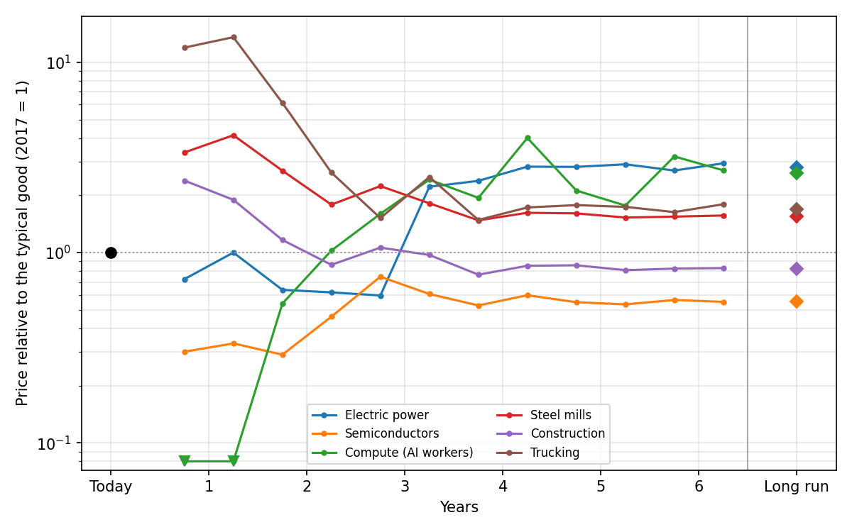
Figure 2. Prices relative to the typical good, in half-year averages. Diamonds on the right are long-run prices.
In the first few years prices follow scarcity. Goods the buildout needs more of than their industries can make, such as trucking, rail freight, and construction, are expensive. Goods made with spare capacity sell at the cost of their inputs, so electricity is cheap, while steel is expensive because the rail freight and trucking it uses are scarce. In the long run, prices converge to values that depend only on the production recipes and the maximum growth rate, which makes them much easier to compute.
These prices should not be taken too seriously, especially early on. As noted earlier, they are very sensitive to the assumptions made. In particular, we are assuming maximum growth and holding consumption fixed at today’s level, but in practice consumption will increase. That will increase the value of consumption goods and all the intermediates required to make them.
Compute prices are probably particularly unreliable. AIs might be valuable for purposes like producing new research, providing new kinds of services such as virtual companions, military systems, or cyber defense, or perhaps even because they are valuable in their own right. These applications would all make compute more valuable, but our model misses them entirely.
The shadow prices also determine the value of existing capital. A factory turns inputs worth \(P_0\) into output worth \(P_1\), and its owner keeps the difference, \(P_1 - P_0\), as profit. The factory is worth all the profit it will make, discounted at the interest rate. Figure 3 shows the value of each kind of capital at the start of the transition, relative to the average dollar of capital.
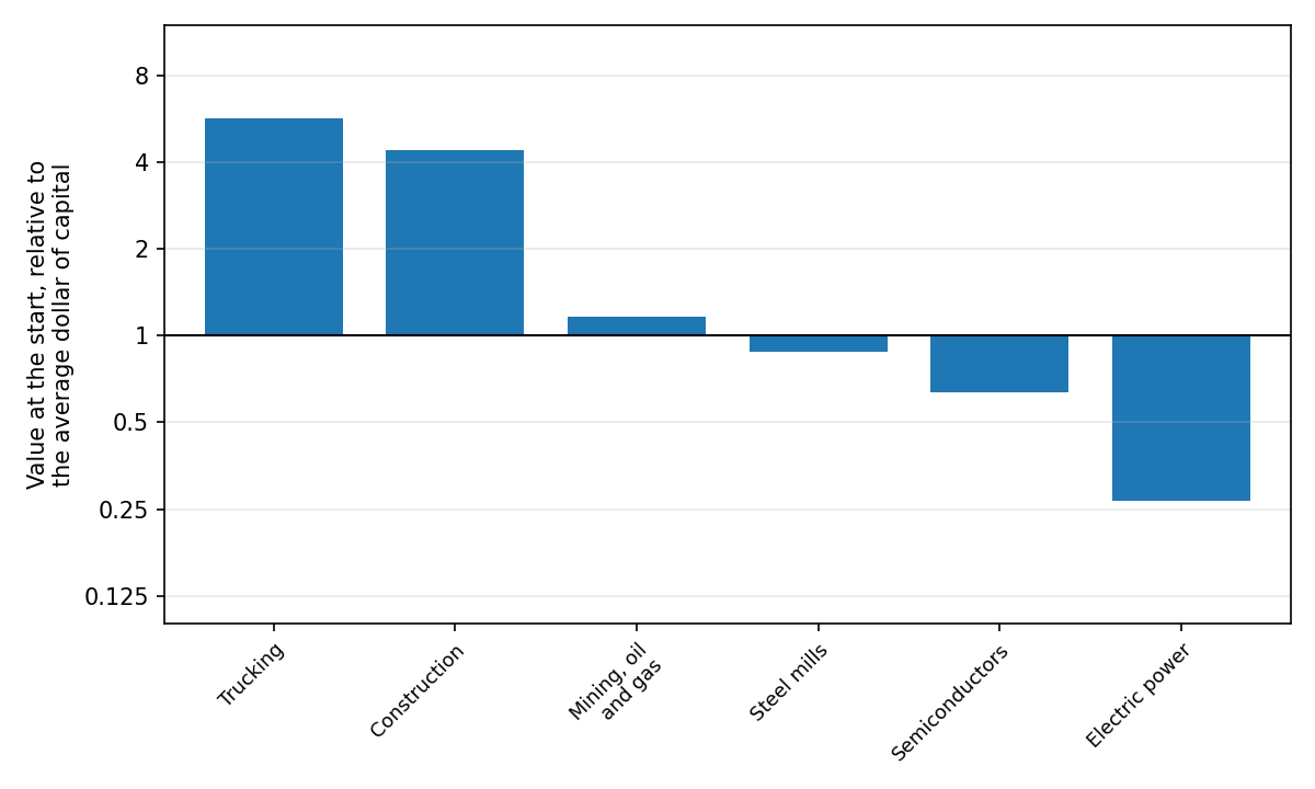
Figure 3. Value of a 2017 dollar of capital at the start, relative to the economy’s average.
These gains and losses happen at the start of the transition. In our toy model, where AI becomes available at time zero, the value of capital changes instantly as the prices of goods and services adjust. After that, anyone who buys a factory pays a price that reflects the profits it will make, so the return on capital matches the interest rate. In the long run, the interest rate equals the growth rate, about 0.6 yr⁻¹ against 0.05 today, because in our model all output beyond today’s consumption is reinvested.
For an industrial takeoff, we are already in a compute overhang
Every AI worker needs compute. In a recent post I estimated that AGI will need between \(10^{13}\) and \(10^{14}\) FLOP/s to do the work of one human. The AI chips already installed in the US, about 22 million H100-equivalents (H100e) by our estimate from Epoch’s chip-sales data, could do the work of 2 billion full-time workers at \(10^{13}\) FLOP/s and 200 million at \(10^{14}\). The US has about 160 million workers, so at either rate today’s chips could already supply the compute to replace every one of them. Even at \(10^{15}\) FLOP/s, they could replace 20 million, about one in eight.
In Part 1 I assumed each AI worker needs \(10^{15}\) FLOP/s, but that estimate falls inside the range above once FLOPs are counted the same way. Part 1 counted the FLOP/s a chip is advertised to deliver, about \(4 \times 10^{15}\) for an H100. The newer post counts the operations the AI actually performs, and an H100 performs about \(2 \times 10^{14}\) a second. Part 1’s \(10^{15}\) FLOP/s is therefore 20 times smaller in the newer post’s terms, about \(5 \times 10^{13}\). I think counting the operations actually performed is the better convention, and I use it in this post.
To check whether chips could still hold back the buildout, we replaced Part 2’s single compute sector with the 34 industries of the AI chip supply chain, from EUV lithography to data centers (see Appendix K.1 for details). Each starts from the capacity the US has today, and today’s imports of chips and chipmaking equipment continue. We assume their plants are built with 24/7 construction substantially optimized by AI, as there’s a strong economic incentive to build quickly. A leading-edge fab then takes a little over a year from investment to output, against about three years today. Figure 4 compares free compute with four rates of compute per AI worker:
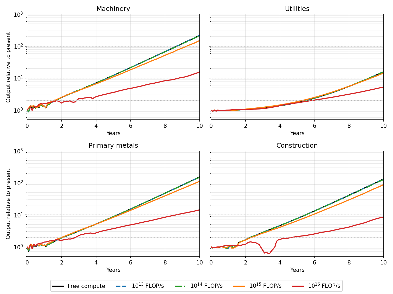
Figure 4. Output relative to present with free compute and at four compute requirements per AI worker.
As Figure 4 shows, below \(10^{15}\) FLOP/s the cost of compute barely affects growth, which is essentially indistinguishable from growth with free compute. At \(10^{15}\) the first two years are about as fast, because the US already has more chips than the buildout needs. Once the economy grows large enough it has to build more chips, which takes resources away from the rest of the buildout, and the economy ends up about half a year behind. At \(10^{16}\) FLOP/s compute slows growth substantially, delaying the buildout by several years.
The US imports most of its leading-edge chips. To test whether this could bottleneck the buildout, we take the pessimistic \(10^{15}\) FLOP/s case and consider three ways the supply of chips could be disrupted:
- No US-made EUV scanners. Only the Dutch company ASML makes the EUV scanners used for the most advanced chips. The US gets ASML’s planned deliveries but can’t build its own, so beyond those it makes AI chips with older DUV lithography. The US doesn’t make the immersion DUV scanners these chips need either (almost all are made by ASML), so to make more than its imports allow, it has to build that industry and the lenses it uses.
- No imported AI hardware. Nearly all AI chips are made by TSMC in Taiwan. The US imports no chips, memory, or servers, but can still import chipmaking tools and materials.
- Chip supply chain cut off. Both of the above, plus no imported chipmaking tools or materials, including DUV scanners. The US can’t add EUV capacity, so new chips use DUV lithography, with scanners, lenses, and materials the US makes itself.
As Figure 5 shows, none of these disruptions make much difference. Losing EUV slows long-run growth slightly, because chips made with DUV lithography use more power, but overall all the effects are small:
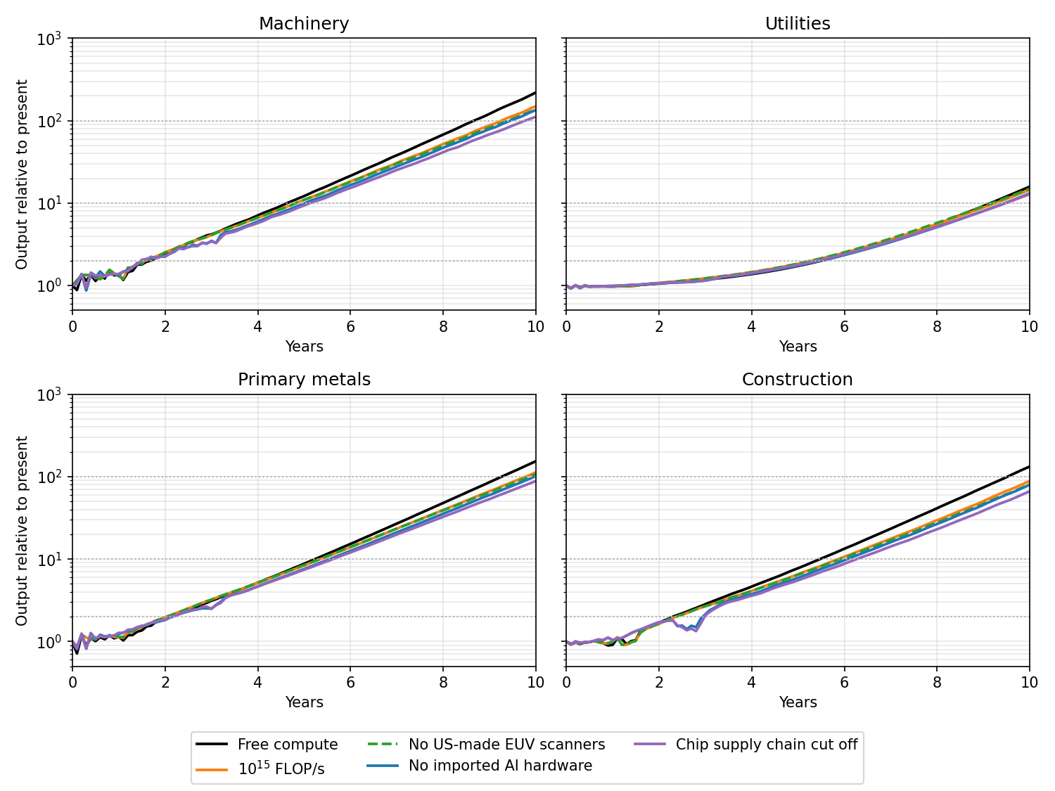
Figure 5. Output relative to present under three scenarios where chip supply is disrupted.
We can also investigate the effect of lags, replacing the fast build times assumed above with today’s, which are two to four years for fabs, chipmaking tools, and data centers. This barely matters if the compute requirement is \(10^{13}\) or \(10^{14}\) FLOP/s, but at \(10^{15}\) it can create substantial delays:
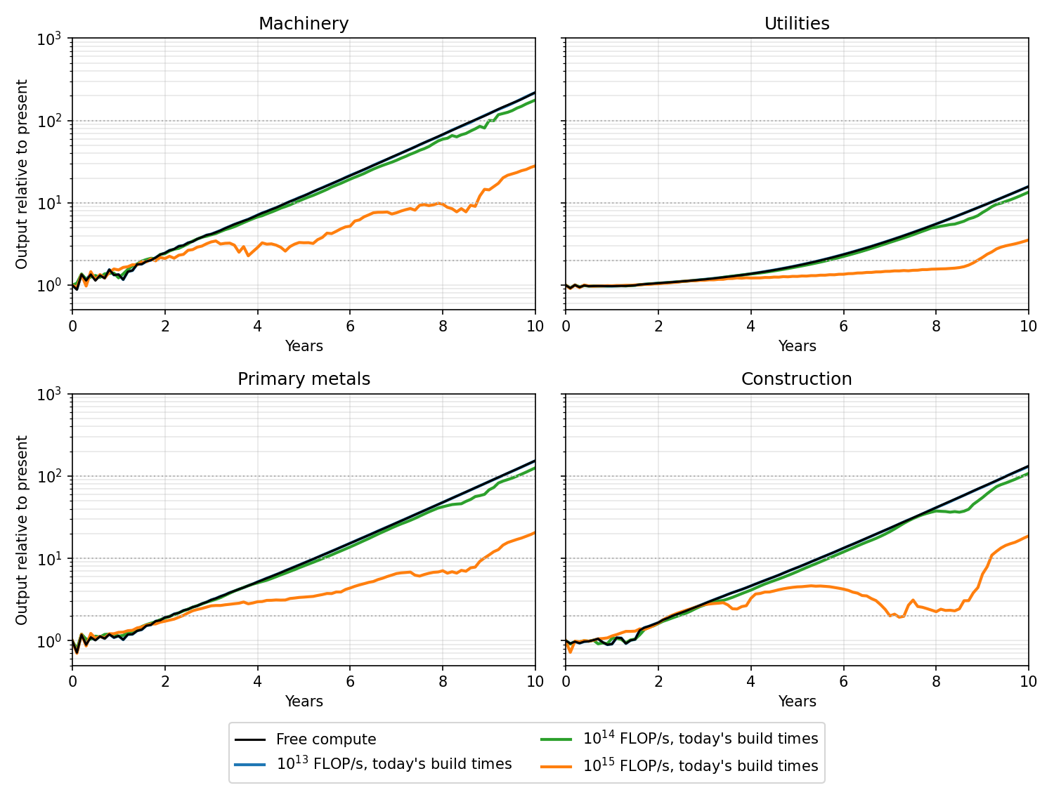
Figure 6. Output relative to present with today’s build times for the chip supply chain.
So far we have assumed that AGI arrives at year zero with a fixed compute requirement. In reality I expect expensive AIs to exist before cheap ones. As a very simple model, suppose the requirement starts at \(10^{18}\) FLOP/s per worker, a thousand times our conservative \(10^{15}\), and falls about threefold each year until it reaches \(10^{13}\) FLOP/s in year ten, after which it stays there (although at this point compute is so cheap that the effect is small). This is slow by recent standards, given that the cost of reaching a given level of AI performance has fallen about 13-fold a year since 2023 (Emberson and Roodman (2026)). Figure 7 shows the results:
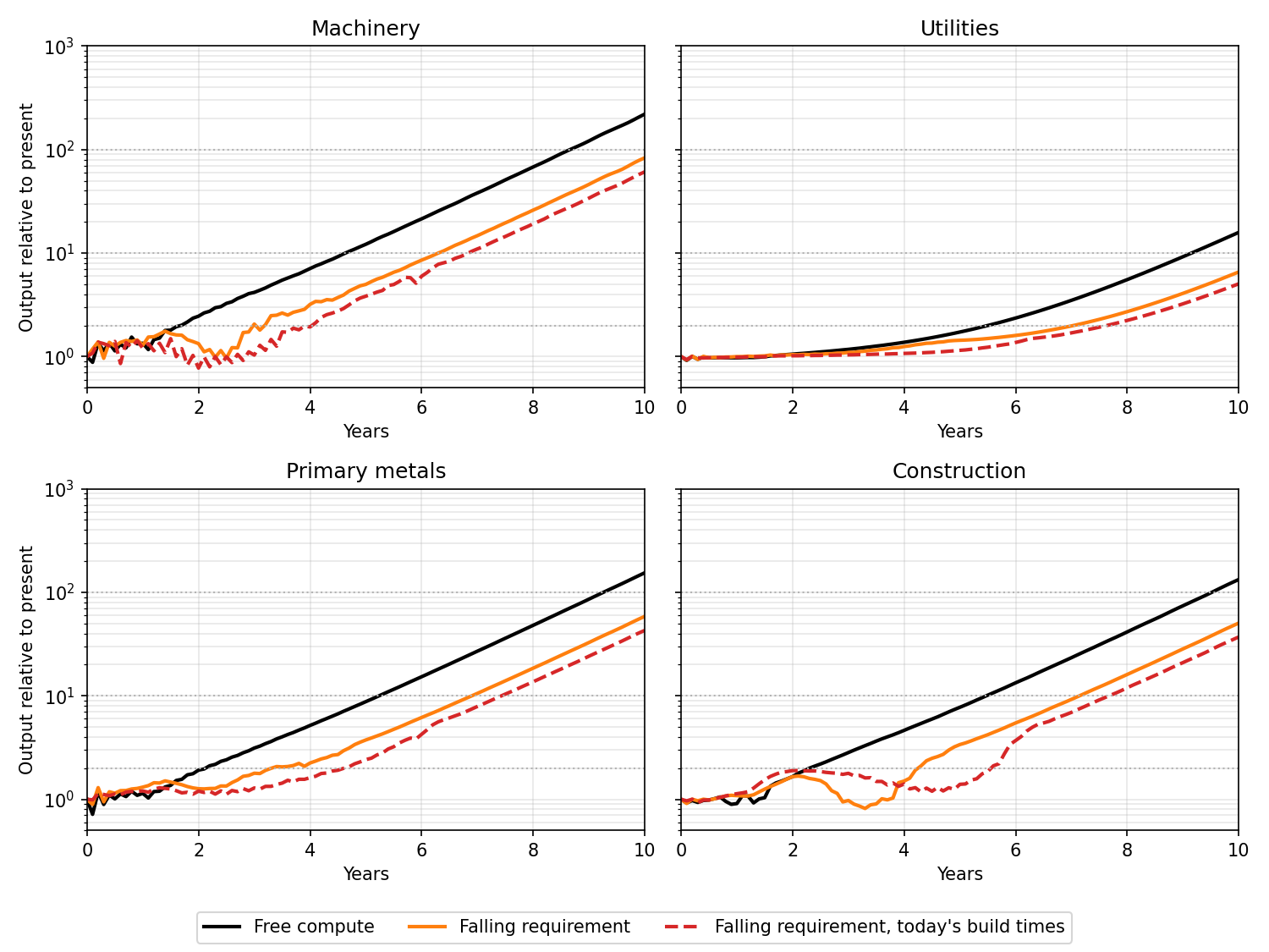
Figure 7. Output relative to present when the compute requirement falls from \(10^{18}\) to \(10^{13}\) FLOP/s over ten years.
The requirement doesn’t reach \(10^{15}\) FLOP/s until year six, yet the economy is less than two years behind a world with free compute from the start. This is because growth is bottlenecked by physical production rather than chips. For the first year or so, even an economy with free compute needs very little AI, because it is busy shifting today’s workers and factories toward building capital. After that, the economy uses what AI it can afford and builds factories and other capacity ahead of time, ready for when AI is cheap. Today’s build times matter much less, because after year four AI gets cheaper faster than the economy grows, so the economy needs fewer chips each year.
All of these calculations assume that compute goes only to the buildout. In practice, some would go to consumption, as discussed in earlier parts, or to compute-heavy uses such as research. If the buildout gets only a fraction of the chips, that is equivalent to raising the compute each worker needs. At \(10^{14}\) FLOP/s, giving the buildout a tenth of the chips is identical to assuming \(10^{15}\) FLOP/s are required but that all chips are used in the industrial buildout, which costs about half a year.
Figure 8 shows the prices of some goods in the chip supply chain in four of these cases, relative to the typical good as in Figure 2. As we can see, they fluctuate, particularly when AGI abruptly becomes available but today’s build times still apply. In that case EUV optics and HBM stacking become extremely, unrealistically valuable. Otherwise, what is scarce and expensive is very sensitive to the assumptions made (and to overall demand for compute, which would include demand from consumption and from R&D). I would not take these results very seriously.
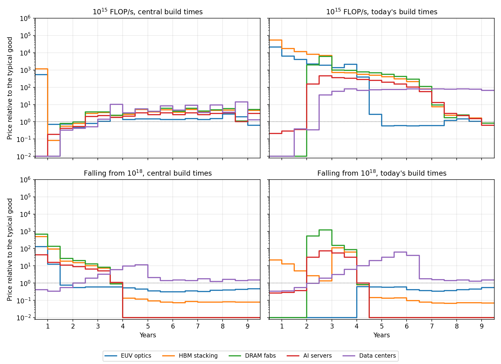
Figure 8. Prices of five goods in the chip supply chain, relative to the typical good.
Robot production does not bottleneck growth
Now let’s turn to the robot supply chain. People often point to components like rare-earth magnets as choke points, because the US makes few of them. To test this, we split Part 2’s single robot sector into six kinds of robot, from humanoids to kits that automate existing vehicles, with numbers set by Part 5’s classification of occupations. Each kind can be built in several ways. Some designs need the scarce parts, mainly rare-earth magnets and precision reducers, while others avoid them with planetary gearboxes, ferrite magnets, or hydraulics. The parts come from 13 industries, each starting from the capacity the US has today. Appendix K.2 gives the details.
As for chips, our central case assumes robot and part factories are built quickly, here in half a year or less. It also lets the economy use any design and keeps today’s imports. Figure 9 compares it with half and double the robots, since our count leaves out how fast robots work and how often they are down, and with today’s build times of one to two years:
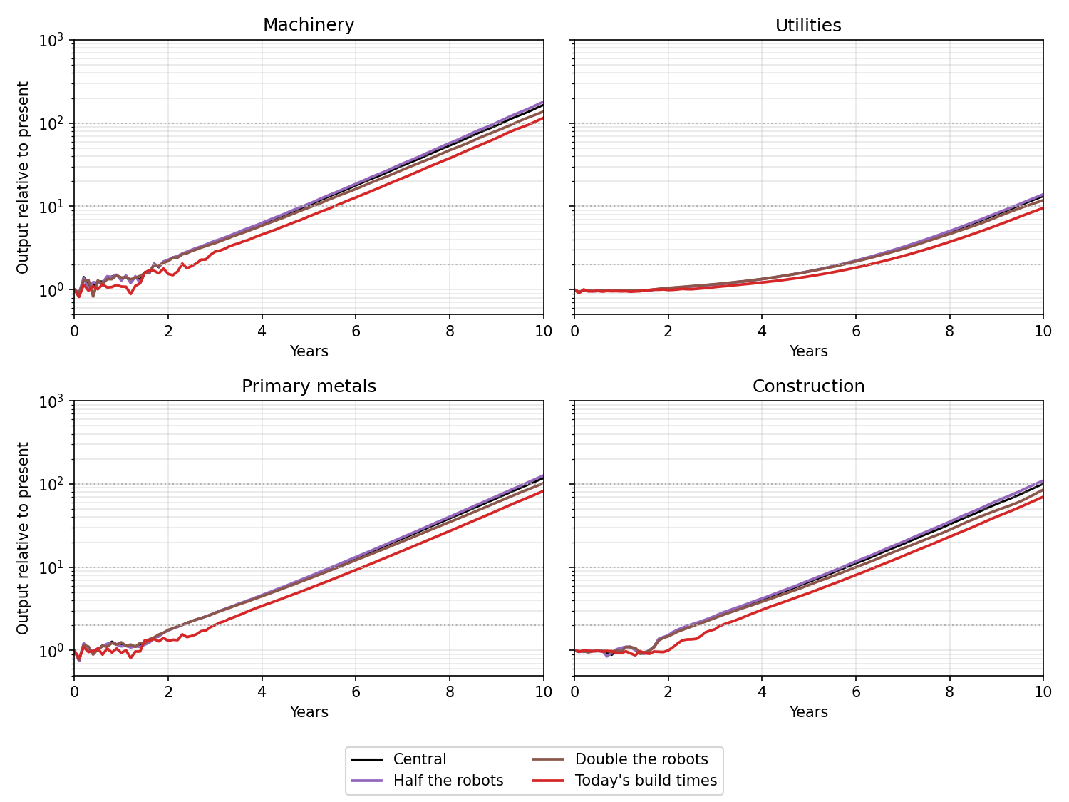
Figure 9. Output relative to present with half and double the robots, and with today’s build times for the robot supply chain.
As we can see, halving or doubling the number of robots barely changes growth, while the pessimistic factory building times delay growth by several months but barely affect the long-run trajectory. This is because robots are a small part of the economy’s capital, about 1% at production cost at first and 4% after ten years.
Now let’s consider the choke points people worry about, with two more scenarios. In the first, the US imports no robots or robot parts. In the second, there is no way around scarce parts, so every robot uses rare-earth magnets and every robot with arms or legs also uses precision reducers. We run the second with both fast and today’s build times. Figure 10 shows the results:
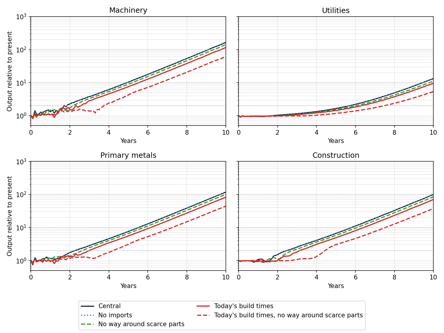
Figure 10. Output relative to present with no robot imports and with no way around scarce parts.
As we can see, losing imports changes nothing. Having no way around scarce parts costs a few months with fast building, but over a year with today’s build times. Imports don’t matter because the US has few robots today, so today’s imports are tiny next to what the buildout needs, and it has to build a robot industry from scratch either way. Scarce parts matter only while their factories are being built, and in the meantime the economy can make robots that avoid them.
Power production does not bottleneck growth
Finally, let’s turn to power. The US imports most of its large power transformers and, by our estimate, about half of its electrical steel and high-voltage breakers, so the grid could be a choke point. To test this, we hold today’s power plants and grid at their current size and supply all new electricity from new gas, coal, nuclear, solar, and wind plants, with storage for solar and wind. Their equipment comes from 57 industries, from transformers and turbines to solar panels and battery cells. Appendix K.3 gives the details.
As for chips and robots, our central case assumes plants and factories are built quickly, gas plants in under a year. It also lets the economy use any design and keeps today’s imports. Figure 11 compares it with the 401-sector model of Figure 1, where electricity comes from a single utilities sector that grows like any other, and with four more cases:
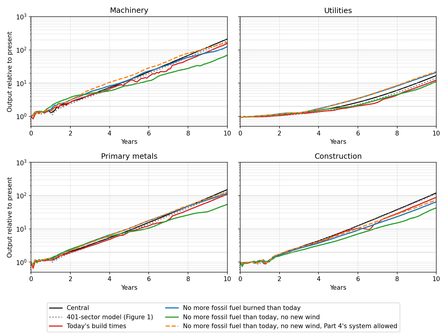
Figure 11. Output relative to present with today’s build times for the power supply chain, and with limits on fossil fuel and wind.
As we can see, splitting up the power sector gives slightly faster growth than the 401-sector model. Adding finer detail and the parts that are hard to scale doesn’t reveal a new choke point. If we instead assume today’s build times, which are somewhat longer than we think could be achieved under strong economic pressure, growth is delayed by about half a year.
Figure 12 shows where electricity comes from after eight years:
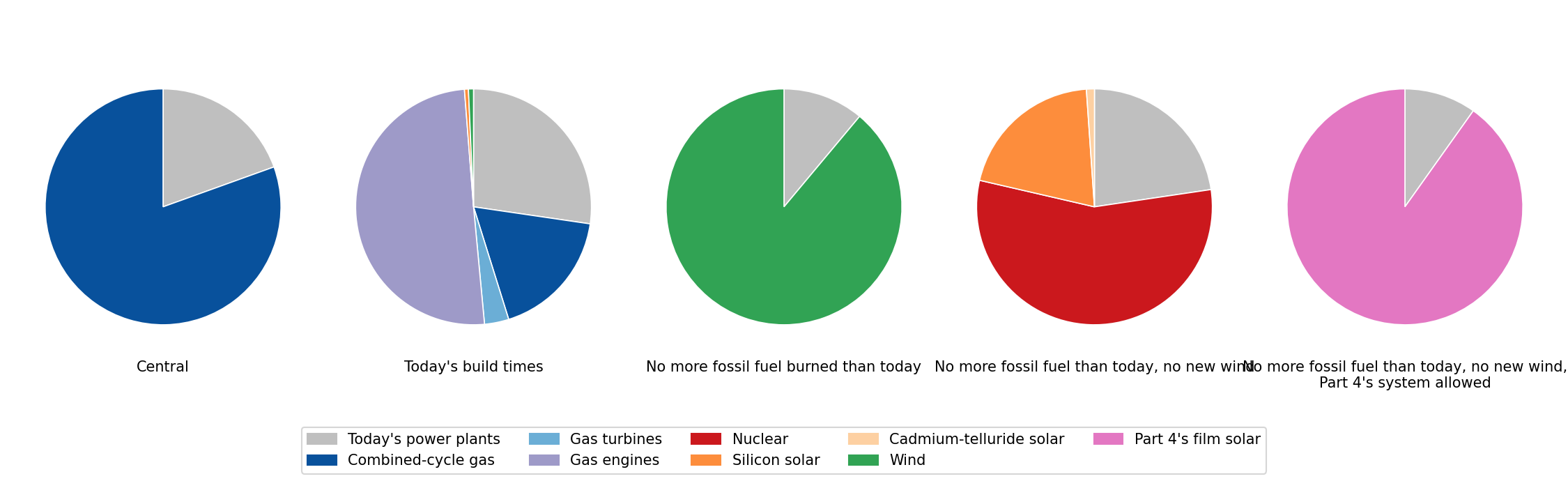
Figure 12. Where electricity comes from after eight years in each case of Figure 11.
In the central case, new power comes almost entirely from combined-cycle gas plants. With today’s build times the economy builds several kinds of gas plant, mostly gas engines, which go up faster. A decade of growth therefore means building a great deal of gas power and burning a lot of gas, and oil and gas extraction grows about thirtyfold in ten years. This is a problem, both because gas supply is limited, which our model ignores, and because it releases huge amounts of carbon dioxide.
If we build no new fossil power plants and hold other fossil fuel burning at today’s level, so that most new uses have to run on electricity, growth slows by about a year and the economy builds wind instead. Utilities grow faster in this case, and machinery does too for about six years, because the uses that switch from fuel need electricity and new electric equipment such as heat pumps. Building so much wind is itself unrealistic, because the buildout soon needs far more wind than the US has good sites for. If the economy also can’t build new wind, it builds a mix of solar and nuclear, and is about two years behind after ten years.
If we instead allow the exotic thin-film solar system we suggested in Part 4, growth recovers most of the way to the gas case.
Appendices
Appendix J: Shadow prices and the value of capital
The transition linear program (Part 2, Appendix D) has a material balance for every good at every time step. The shadow price \(p_i(t)\) of each balance is the gain in the planner’s objective from one more unit of good \(i\) at time \(t\). Prices at every date are in the same units, so they are present values and already include discounting. We quote every price relative to the typical good, the output-weighted median of the 401 industries.
Wherever industry \(j\) is producing, its price equals the cost of its inputs plus a rent,
\[p_j(t) = \sum_i p_i(t) A_{ij} + \mu_j(t),\]where \(\mu_j(t) \geq 0\) is the shadow price of \(j\)’s capacity. The rent is zero whenever \(j\) has spare capacity, so its good sells at the cost of its inputs. A good the economy makes more of than it uses has a price of zero.
We measure capital in 2017 dollars. A unit of capital in industry \(j\) is worth the rents it will earn, less the cost of replacing its wear,
\[V_j(t) = \sum_{s \geq t} \left[ c_j\, \mu_j(s) - \sum_i p_i(s)\, \hat\Delta_{ij} \right] \Delta t ,\]where \(c_j\) is its yearly output and \(\hat\Delta_{ij}\) its yearly wear of good \(i\). The sum needs no discounting, since the prices are present values. Wherever \(j\) is building, a unit of capital finished at \(t + \tau\) is also worth what it cost at \(t\),
\[V_j(t + \tau) = \sum_i p_i(t)\, \hat B_{ij},\]where \(\tau\) is the construction lag and \(\hat B_{ij}\) the amount of good \(i\) in a unit of capital. The sum would need the value of capital at the end of the run, so instead we fix \(V_j\) by this condition wherever \(j\) builds and use the sum to carry it back to earlier times.
In the long run the economy grows at its maximum rate \(\lambda\), relative prices stop changing, and every price falls at \(\lambda\), so the interest rate is \(\lambda\). Every industry earns the same return on the current cost of its capital, \(\lambda e^{\lambda \tau}\). The extra factor \(e^{\lambda \tau}\) arises because capital is paid for \(\tau\) before it produces. Long-run prices therefore satisfy
\[p_j = \sum_i p_i A_{ij} + \sum_i p_i \left( \lambda e^{\lambda \tau} B_{ij} + \Delta_{ij} \right) / m_j ,\]where \(m_j\) is the utilization multiplier.
Appendix K: The compute, robot and power supply chains
K.1 Compute
We replace Part 2’s single compute sector with 34 industries, from EUV scanners and their parts through fabs, packaging, and servers to data centers. Six of them form a second path that makes AI chips without EUV. Figure 13 shows how they connect:
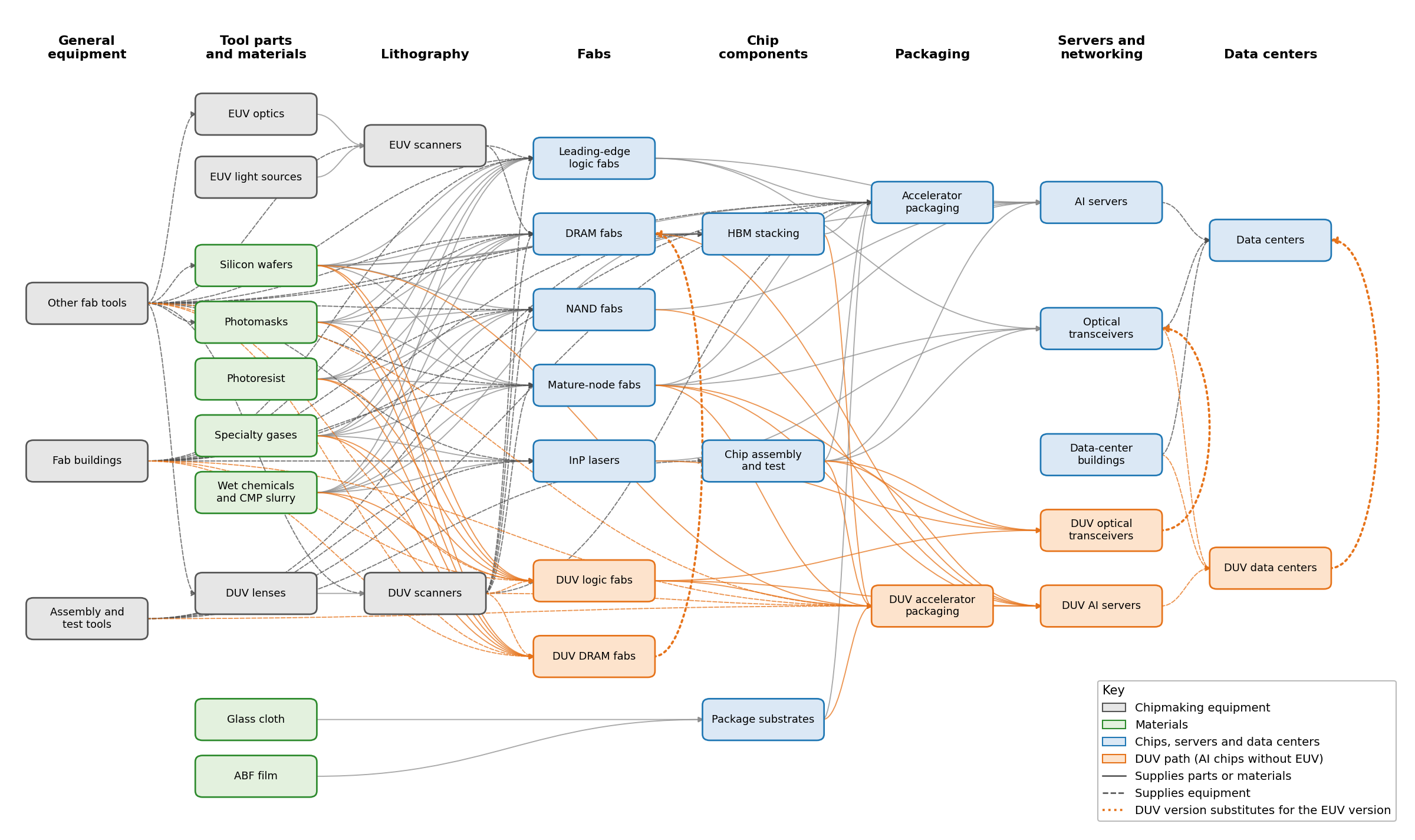
Figure 13. The 34 industries of the AI chip supply chain in the model, and which supply which.
Each industry’s recipe, capital, US capacity, and build times were researched by Claude Opus 5.5 from public sources, such as company filings, trade press, and industry analysts. We value each new industry’s output at production cost, without the margins of chip designers, foundries, and toolmakers. Since each good is valued in the same units as an input and output, the choice of units doesn’t physically matter. At production cost, one H100e of capacity needs about $8,200 of capital in 2017 dollars, about four-fifths of it the data hall’s building, power, and cooling.
An H100 performs about \(2 \times 10^{14}\) FLOP/s around the clock, while a human works 2,000 hours a year, so each \(10^{15}\) FLOP/s per worker needs just over a single H100e. As in Part 2, every industry requires compute in proportion to its current labor requirements. Each industry starts from today’s US capacity, including the 22.4 million H100e installed at the end of September 2026, and imports continue at today’s levels.
Every industry from Part 2 includes a half-year construction lag. The new industries’ delays from investment to output cover building the plant, installing and qualifying its equipment, and ramping up. The central case assumes 24/7 construction optimized by AI, and the other case today’s build times:
| Industry | Central (yr) | Today’s (yr) |
|---|---|---|
| EUV scanners | 0.8 | 3.3 |
| EUV optics | 0.9 | 4.0 |
| Silicon wafers | 0.8 | 3.0 |
| Leading-edge logic fabs | 1.2 | 3.0 |
| DRAM fabs | 1.2 | 3.0 |
| HBM stacking | 0.9 | 2.8 |
| Chip packaging | 1.0 | 2.6 |
| AI servers | 0.5 | 2.0 |
| Data centers | 0.5 | 2.0 |
Without EUV, AI chips are made on 7 nm-class DUV processes, which use about 70% more power to do compute.
K.2 Robots
We replace Part 2’s single robot sector with six kinds of robot and add an additional 13 industries making critical inputs for these robots, including rare-earth magnets, precision reducers and screws, machines that cut and grind their gears, servo motors, and force-torque sensors. Each kind of robot can be built in several designs, some of which avoid the scarce parts. Figure 14 shows how they connect:
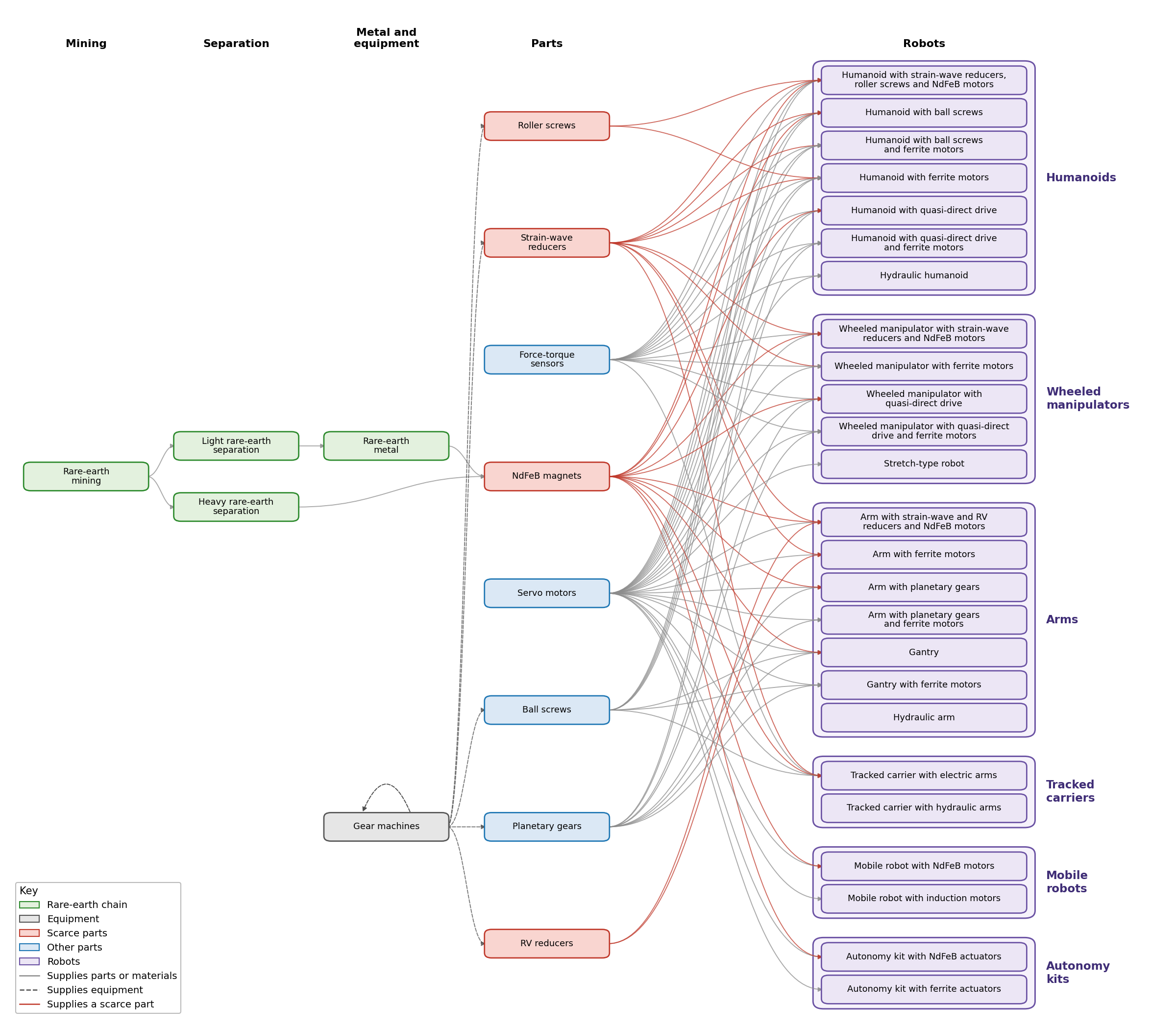
Figure 14. The robot supply chain in the model: the 13 industries that make robot parts, the 25 robot designs grouped by kind, and which supply which.
As for compute, each industry’s recipe, capital, US capacity, and build times were researched by Claude Opus 5.5 from public sources, and each good is valued at production cost. Labor is valued at US wages, including the hours of the Chinese and Japanese plants the recipes are measured in, which makes reducers and screws cost about twice their Chinese prices. For simplicity, we assume that robots do not carry their own compute, and instead this compute is costed with the data centers.
Part 2 assumed that one robot replaces four full-time workers. Here we use Part 5’s classification of occupations to count the positions that need a robot body, and give each a robot of the kind its work needs. Every vehicle and mobile machine also gets an autonomy kit. Wheeled manipulators are two arms on a wheeled base, tracked carriers are small tracked machines with a boom and two arms, and autonomy kits fit existing vehicles and machines with the sensors and actuators an AI needs to drive them. For 2017’s output this gives 43 million robots, which at production cost would be 1.2% of the capital needed for that output.
The new industries’ delays from investment to output are:
| Industry | Central (yr) | Today’s (yr) |
|---|---|---|
| Rare-earth mining | 0.4 | 2.3 |
| Rare-earth separation | 0.5 | 1.9 |
| Rare-earth metal | 0.4 | 1.8 |
| NdFeB magnets | 0.5 | 1.9 |
| Gear machines | 0.4 | 1.6 |
| Strain-wave reducers, planetary gears, and roller and ball screws | 0.4 | 1.4 |
| RV reducers | 0.5 | 1.5 |
| Servo motors | 0.4 | 1.5 |
| Force-torque sensors | 0.3 | 1.3 |
| Arms, humanoids, and wheeled manipulators | 0.3 | 1.5 |
| Tracked carriers | 0.3 | 1.4 |
| Mobile robots and autonomy kits | 0.3 | 1.3 |
K.3 Power
We hold Part 2’s three electricity producers at today’s capital, so today’s power plants and grid keep running and replace what wears out but don’t expand. All new electricity comes from nine designs of power plant through a new grid, and their equipment, storage, and fuel come from 57 industries. Figure 15 shows how they connect:
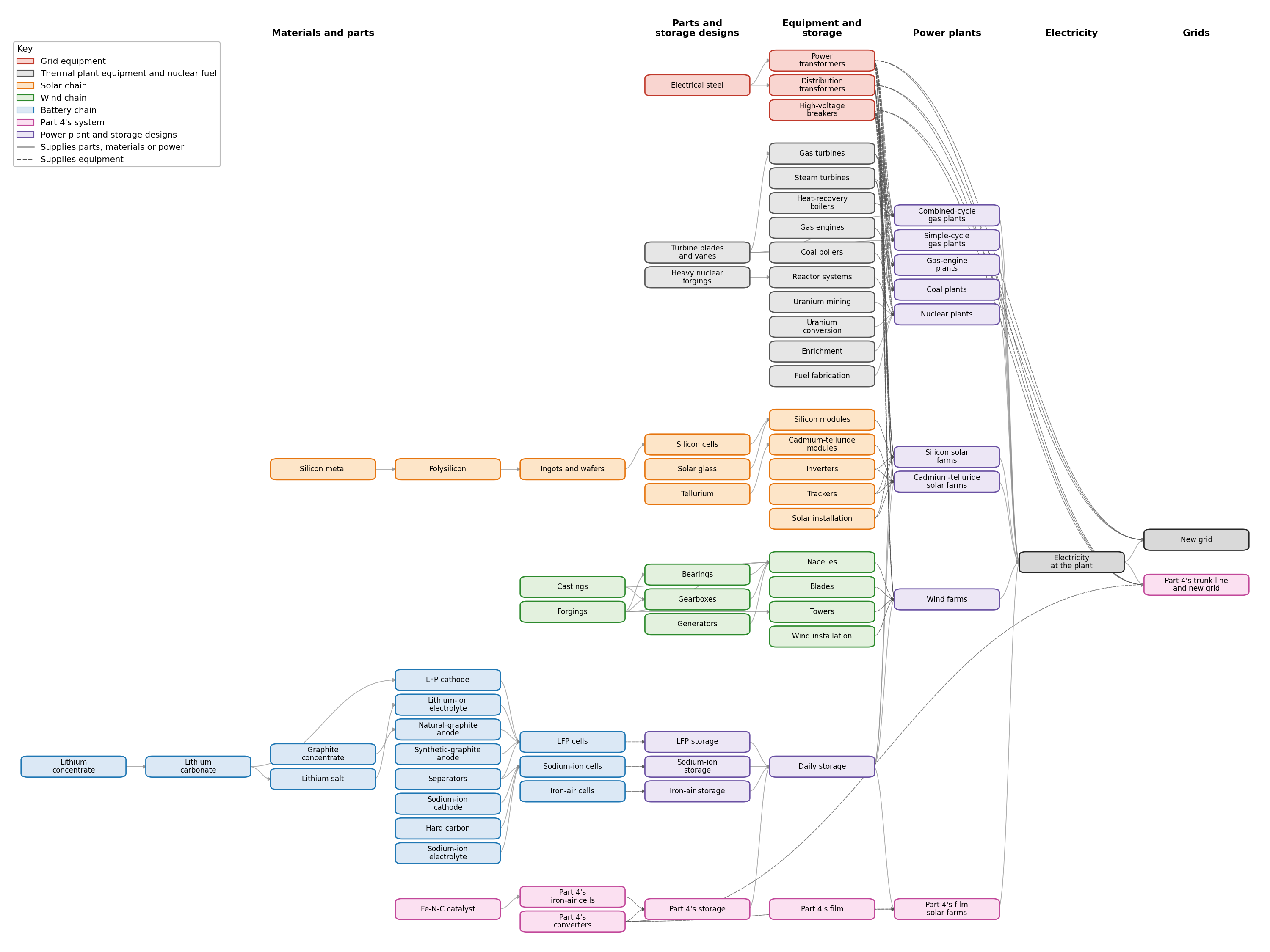
Figure 15. The power supply chain in the model: the industries that make plant equipment, storage, and fuel, the plant designs, and the two grids.
As for compute and robots, each industry’s recipe, capital, US capacity, and build times were researched by Claude Opus 5.5 from public sources, and each good is valued at production cost. Solar and wind plants carry enough batteries to deliver flat output through each day, but none for longer lulls or for winter. Fuel that is burned, for example in vehicles or for building heat, can switch to electric equipment, while fuel used as feedstock can’t. Oil, gas, and coal supply grow like any other industry, with no depletion.
Part 4’s system enters as three designs (its film solar farms, trunk line, and iron-air storage), made by four new industries that start from nothing. We firm its film like the other solar designs, which takes 25 hours of storage per unit of delivered power against Part 4’s 12, because Part 4 assumed clear days. Its trunk runs 240 km rather than 1,000, and since Part 4 designed nothing below the trunk, it feeds the new grid’s lower-voltage network.
The delays from investment to output are:
| Plant or industry | Central (yr) | Today’s (yr) |
|---|---|---|
| Combined-cycle gas | 0.8 | 2.4 |
| Simple-cycle gas | 0.6 | 1.7 |
| Gas engines | 0.4 | 1.2 |
| Coal | 1.3 | 3.3 |
| Nuclear | 2.3 | 4.5 |
| Solar | 0.2 | 1.1 |
| Onshore wind | 0.2 | 1.1 |
| Part 4’s film solar | 0.1 | — |
| New grid | 0.5 | 2.0 |
| Power transformers | 1.1 | 3.3 |
| Electrical steel | 1.6 | 4.5 |
| High-voltage breakers | 0.8 | 2.5 |
| Gas turbines | 1.1 | 3.0 |